手把手带你入门最简单的图像处理和人脸识别过程
文章目录
前言
如果说NLP是人工智能皇冠上的明珠,CV可以说是人工智能的眼睛。本文主要介绍了图像处理和人脸识别的原理和相关理论,之后通过代码实操展示了图像处理的和人脸识别的流程。
一、图像处理
1.图像处理内容
• 图像的识别分类
2.常用算法
图像的几何变换(图像畸变校正、图像缩放:双线性插值、旋转、拼接)
图像变换(傅立叶、余弦、沃尔什-哈达玛、K-L变换、小波变换)
图像频域处理(增强算法:高频率提升、同态滤波;平滑去噪:低通滤波)
Python 计算机视觉(八)—— OpenCV 进行图像增强_一马归一码的博客-CSDN博客_opencv 图像增强(图像增强)
3.图像数据增强
图像数据增强是一种技术,通过在现有图像数据集上执行一系列变换来创建新的图像数据集,从而扩展原始图像数据集。它的目的是让机器学习模型能够更好地捕捉图像的复杂性,更好地泛化到新的数据集上。常见的图像数据增强技术包括旋转、缩放、裁剪、反转、颜色变换等。
深度学习中图像数据增强:
图像增强代码演示:
# 图像增强算法,图像锐化算法
# 1)基于直方图均衡化 2)基于拉普拉斯算子 3)基于对数变换 4)基于伽马变换 5)CLAHE 6)retinex-SSR 7)retinex-MSR
# 其中,基于拉普拉斯算子的图像增强为利用空域卷积运算实现滤波
# 基于同一图像对比增强效果
# 直方图均衡化:对比度较低的图像适合使用直方图均衡化方法来增强图像细节
# 拉普拉斯算子可以增强局部的图像对比度
# log对数变换对于整体对比度偏低并且灰度值偏低的图像增强效果较好
# 伽马变换对于图像对比度偏低,并且整体亮度值偏高(对于相机过曝)情况下的图像增强效果明显

import cv2
import numpy as np
import matplotlib.pyplot as plt


# 直方图均衡增强
def hist(image):
    r, g, b = cv2.split(image)
    r1 = cv2.equalizeHist(r)
    g1 = cv2.equalizeHist(g)
    b1 = cv2.equalizeHist(b)
    image_equal_clo = cv2.merge([r1, g1, b1])
    return image_equal_clo


# 拉普拉斯算子
def laplacian(image):
    kernel = np.array([[0, -1, 0], [-1, 5, -1], [0, -1, 0]])
    image_lap = cv2.filter2D(image, cv2.CV_8UC3, kernel)
    return image_lap


# 对数变换
def log(image):
    image_log = np.uint8(np.log(np.array(image) + 1))
    cv2.normalize(image_log, image_log, 0, 255, cv2.NORM_MINMAX)
    # 转换成8bit图像显示
    cv2.convertScaleAbs(image_log, image_log)
    return image_log


# 伽马变换
def gamma(image):
    fgamma = 2
    image_gamma = np.uint8(np.power((np.array(image) / 255.0), fgamma) * 255.0)
    cv2.normalize(image_gamma, image_gamma, 0, 255, cv2.NORM_MINMAX)
    cv2.convertScaleAbs(image_gamma, image_gamma)
    return image_gamma


# 限制对比度自适应直方图均衡化CLAHE
def clahe(image):
    b, g, r = cv2.split(image)
    clahe = cv2.createCLAHE(clipLimit=2.0, tileGridSize=(8, 8))
    b = clahe.apply(b)
    g = clahe.apply(g)
    r = clahe.apply(r)
    image_clahe = cv2.merge([b, g, r])
    return image_clahe


def replaceZeroes(data):
    min_nonzero = min(data[np.nonzero(data)])
    data[data == 0] = min_nonzero
    return data


# retinex SSR
def SSR(src_img, size):
    L_blur = cv2.GaussianBlur(src_img, (size, size), 0)
    img = replaceZeroes(src_img)
    L_blur = replaceZeroes(L_blur)

    dst_Img = cv2.log(img/255.0)
    dst_Lblur = cv2.log(L_blur/255.0)
    dst_IxL = cv2.multiply(dst_Img, dst_Lblur)
    log_R = cv2.subtract(dst_Img, dst_IxL)

    dst_R = cv2.normalize(log_R,None, 0, 255, cv2.NORM_MINMAX)
    log_uint8 = cv2.convertScaleAbs(dst_R)
    return log_uint8


def SSR_image(image):
    size = 3
    b_gray, g_gray, r_gray = cv2.split(image)
    b_gray = SSR(b_gray, size)
    g_gray = SSR(g_gray, size)
    r_gray = SSR(r_gray, size)
    result = cv2.merge([b_gray, g_gray, r_gray])
    return result


# retinex MMR
def MSR(img, scales):
    weight = 1 / 3.0
    scales_size = len(scales)
    h, w = img.shape[:2]
    log_R = np.zeros((h, w), dtype=np.float32)

    for i in range(scales_size):
        img = replaceZeroes(img)
        L_blur = cv2.GaussianBlur(img, (scales[i], scales[i]), 0)
        L_blur = replaceZeroes(L_blur)
        dst_Img = cv2.log(img/255.0)
        dst_Lblur = cv2.log(L_blur/255.0)
        dst_Ixl = cv2.multiply(dst_Img, dst_Lblur)
        log_R += weight * cv2.subtract(dst_Img, dst_Ixl)

    dst_R = cv2.normalize(log_R,None, 0, 255, cv2.NORM_MINMAX)
    log_uint8 = cv2.convertScaleAbs(dst_R)
    return log_uint8


def MSR_image(image):
    scales = [15, 101, 301]  # [3,5,9]
    b_gray, g_gray, r_gray = cv2.split(image)
    b_gray = MSR(b_gray, scales)
    g_gray = MSR(g_gray, scales)
    r_gray = MSR(r_gray, scales)
    result = cv2.merge([b_gray, g_gray, r_gray])
    return result


if __name__ == "__main__":
    image = cv2.imread("example.jpg")
    image_gray = cv2.cvtColor(image, cv2.COLOR_BGR2GRAY)

    plt.subplot(4, 2, 1)
    plt.imshow(image)
    plt.axis('off')
    plt.title('Offical')

    # 直方图均衡增强
    image_equal_clo = hist(image)

    plt.subplot(4, 2, 2)
    plt.imshow(image_equal_clo)
    plt.axis('off')
    plt.title('equal_enhance')

    # 拉普拉斯算法增强
    image_lap = laplacian(image)

    plt.subplot(4, 2, 3)
    plt.imshow(image_lap)
    plt.axis('off')
    plt.title('laplacian_enhance')

    # LoG对象算法增强
    image_log = log(image)

    plt.subplot(4, 2, 4)
    plt.imshow(image_log)
    plt.axis('off')
    plt.title('log_enhance')

    # 伽马变换
    image_gamma = gamma(image)

    plt.subplot(4, 2, 5)
    plt.imshow(image_gamma)
    plt.axis('off')
    plt.title('gamma_enhance')

    # CLAHE
    image_clahe = clahe(image)

    plt.subplot(4, 2, 6)
    plt.imshow(image_clahe)
    plt.axis('off')
    plt.title('CLAHE')

    # retinex_ssr
    image_ssr = SSR_image(image)

    plt.subplot(4, 2, 7)
    plt.imshow(image_ssr)
    plt.axis('off')
    plt.title('SSR')

    # retinex_msr
    image_msr = MSR_image(image)

    plt.subplot(4, 2, 8)
    plt.imshow(image_msr)
    plt.axis('off')
    plt.title('MSR')

    plt.show()
处理之后的图片:
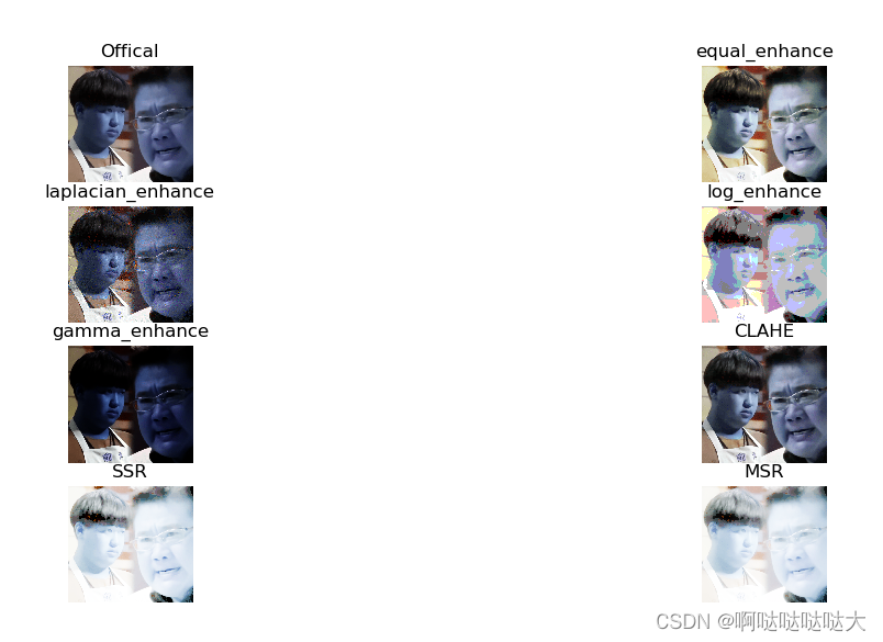
1)基于直方图均衡化 2)基于拉普拉斯算子 3)基于对数变换 4)基于伽马变换 5)CLAHE 6)retinex-SSR 7)retinex-MSR
1.直方图均衡化:对比度较低的图像适合使用直方图均衡化方法来增强图像细节
2.拉普拉斯算子可以增强局部的图像对比度
3.log对数变换对于整体对比度偏低并且灰度值偏低的图像增强效果较好
4.伽马变换对于图像对比度偏低,并且整体亮度值偏高(对于相机过曝)情况下的图像增强效果明显
56.CLAHE和retinex的效果均较好
在输出中使用cv2.imread()读取图像时,默认彩色图像的三通道顺序为B、G、R,这与我们所熟知的RGB中的R通道和B通道正好互换位置了。而使用plt.imshow()函数却默认显示图像的通道顺序为R、G、B,导致图像出现色差发蓝。
二、人脸识别
1.人脸识别内容
·人脸检测(Face Detection):目标识别
·人脸配准(Face Alignment) 人脸上五官关键点坐标,数量是预先设定好的一个固定数值,常见的有5点、68点、90点等等
·人脸提特征(Face Feature Extraction)将一张人脸图像转化为可以表征人脸特点的特征,具体表现形式为一串固定长度的数值。首先将五官关键点坐标进行旋转、缩放等等操作来实现人脸对齐,然后在提取特征并计算出数值串。
·人脸比对(Face Compare):算法实现的目的是衡量两个人脸之间相似度。人脸比对算法的输入是两个人脸特征人脸特征由前面的人脸提特征算法获得,输出是两个特征之间的相似度。
·人脸匹配:人脸匹配人脸匹配就是给定任意两张人脸图像,判断这两张人脸图像中的人脸是否属于同一个人。
人脸匹配过程:识别出每张图像中的人脸,找到人脸所在的位置,接着对人脸提取特征,最后对比不同人脸的特征之间的距离,如果距离小于某个阈值则认为是同一张人脸,否则就认为是不同的人脸。
人脸匹配模式:
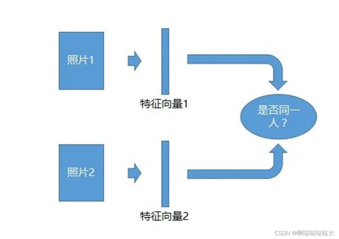
•1:1 认证比对
2.对比核心流程
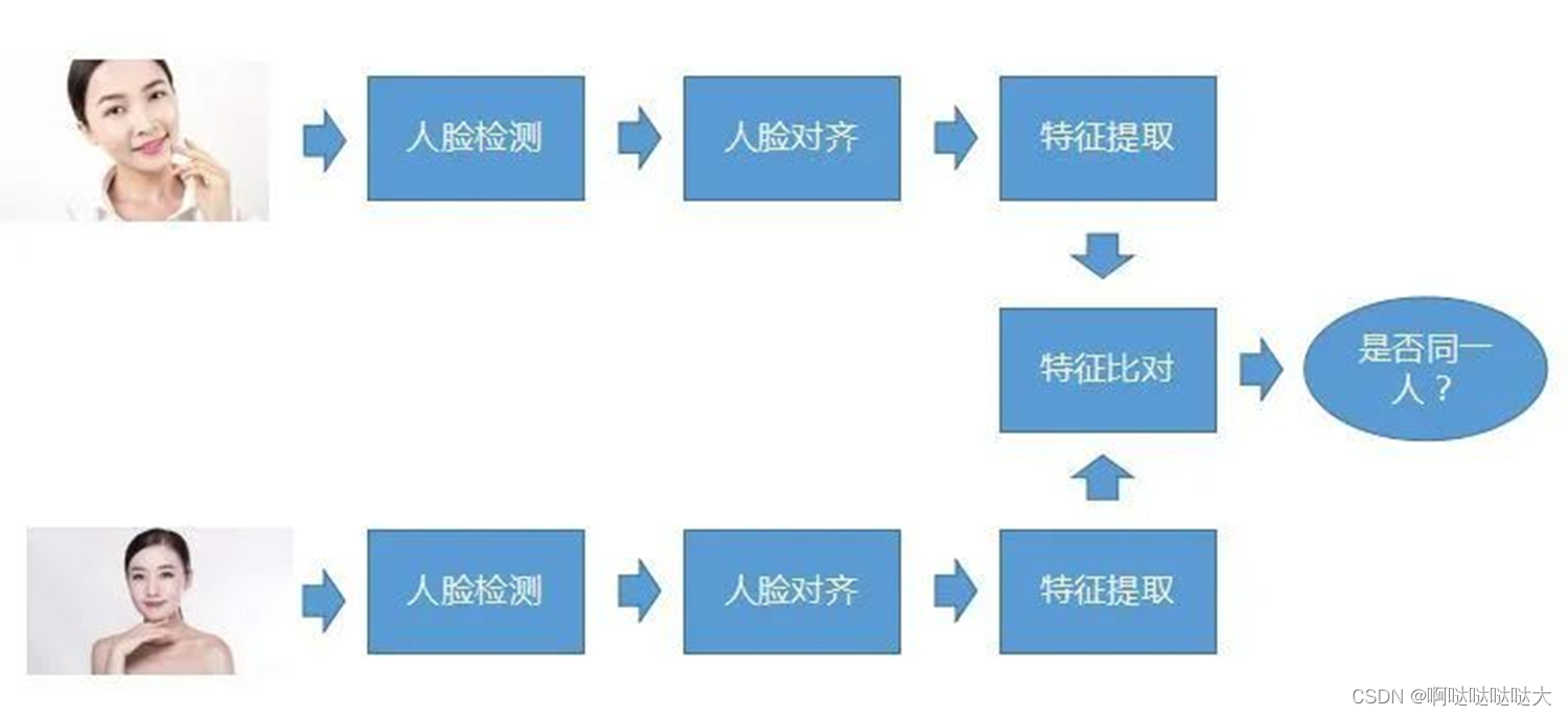
首先人脸检测,第二步做人脸对齐,第三步做特征提取,这是对每一张照片都要做的这三步,当要去做比对的时候就把提取的特征做比对,然后确定这两个脸是不是属于同一个人。
人脸检测:
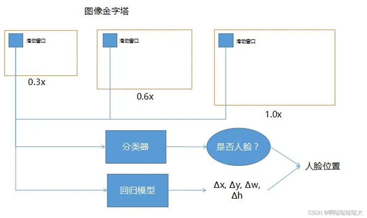
分类器是指看滑动窗口每一个滑到的位置去判断是否是人脸,把滑动窗口放到回归模型里,即可帮助修正人脸检测的精确度。输入的是滑动窗口,输出时如果里面有人脸,应该向哪边修正,以及它需要修正多少,所以Δx, Δy, Δw, Δh,就是它的坐标以及它的宽和高大概修正多少,最后能比较精确的找到人脸
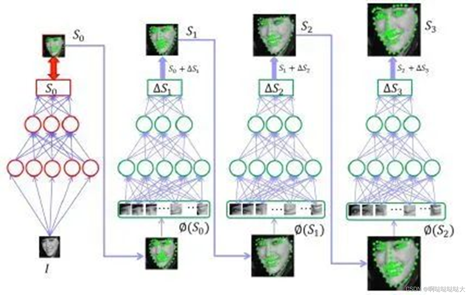
人脸特征提取算法:以前的传统方法是所谓的局部纹理模型,全局纹理模型,形状回归模型之类的这些都有。现在比较流行的就是用深度的卷积神经网络或者循环神经网络,或者3DMM参数的卷积神经网络。所谓3DMM参数的话就是有三维的信息在里面,然后有级联的深度神经网络。
人脸比对的方法:
•主流的方法就是深度的方法,即深度卷积神经网络,这个网络一般来说是用DCNN去代替前面的那些特征抽取方法,即把一张图上面,一个人脸上面的一些各个不同的特征弄出来,DCNN里面有很多参数,这个参数是学出来的,不是人告诉他的,学出来的话相当于能比人总结出来的这些会更好。然后得到的一组特征一般现在的维度可能是128维、256维或者512维、1024维,然后做对比. 判断特征向量之间的距离,一般使用欧氏距离或余弦相似度。人脸比对的评价指标同样分为速度与精度,速度包括单张人脸特征向量计算时间和比对速度。精度包括ACC和ROC。
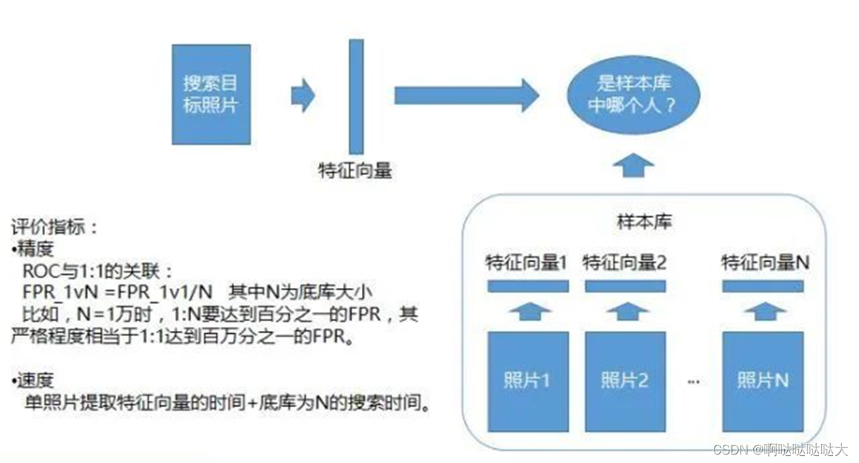
•普通比对是一个简单的运算,是做两个点的距离,可能只需要去做一次内积,就是两个向量的内积,但当人脸识别遇到1:N对比时,当那个N库很大的时候,拿到一张照片要去N库里面做搜索的时候,搜索的次数会非常多,比如N库一百万,可能要搜索一百万次,一百万次的话就相当于要做一百万次的比对,这个时候的话对于总时间还是有要求的,所以就会有各种各样的技术对这种比对进行加速
3.算法
dlib:

facenet、arcface等
三、代码及实操展示
代码都是基于face_recognition库实现的,比较简单,安装此库的时候注意要有dlib库和opencv-python,然后还要有cmake库,安装的时候也踩了一些坑,值得注意的是库对32位和64位的python比较敏感,然后注意环境配置
关键点识别:
from PIL import Image, ImageDraw
import face_recognition

# Load the jpg file into a numpy array
image = face_recognition.load_image_file("biden.jpg")

# Find all facial features in all the faces in the image
face_landmarks_list = face_recognition.face_landmarks(image)

print("I found {} face(s) in this photograph.".format(len(face_landmarks_list)))

# Create a PIL imagedraw object so we can draw on the picture
pil_image = Image.fromarray(image)
d = ImageDraw.Draw(pil_image)

for face_landmarks in face_landmarks_list:

    # Print the location of each facial feature in this image
    for facial_feature in face_landmarks.keys():
        print("The {} in this face has the following points: {}".format(facial_feature, face_landmarks[facial_feature]))

    # Let's trace out each facial feature in the image with a line!
    for facial_feature in face_landmarks.keys():
        d.line(face_landmarks[facial_feature], width=5)

# Show the picture
pil_image.show()
识别效果:

输出的关键点坐标:I found 1 face(s) in this photograph.
The chin in this face has the following points: [(182, 120), (184, 135), (187, 150), (191, 165), (197, 178), (207, 189), (219, 198), (230, 205), (243, 205), (255, 201), (264, 191), (272, 179), (278, 167), (281, 153), (281, 140), (281, 126), (280, 113)]
The left_eyebrow in this face has the following points: [(194, 112), (199, 105), (208, 103), (218, 104), (226, 108)]
The right_eyebrow in this face has the following points: [(241, 107), (249, 103), (257, 101), (266, 101), (272, 107)]
The nose_bridge in this face has the following points: [(235, 119), (236, 128), (237, 137), (238, 146)]
The nose_tip in this face has the following points: [(227, 152), (233, 153), (238, 154), (244, 152), (248, 150)]
The left_eye in this face has the following points: [(205, 122), (210, 119), (216, 120), (223, 124), (217, 125), (210, 125)]
The right_eye in this face has the following points: [(247, 122), (252, 117), (258, 116), (264, 118), (259, 121), (253, 122)]
The top_lip in this face has the following points: [(215, 169), (223, 166), (233, 164), (239, 165), (245, 163), (254, 163), (262, 165), (259, 166), (246, 166), (239, 167), (233, 167), (217, 169)]
The bottom_lip in this face has the following points: [(262, 165), (256, 179), (247, 186), (240, 187), (234, 187), (223, 182), (215, 169), (217, 169), (233, 181), (240, 181), (246, 180), (259, 166)]
一共是九个关键点。
人脸化妆:
很简单的进行化妆
from PIL import Image, ImageDraw
import face_recognition

# Load the jpg file into a numpy array
image = face_recognition.load_image_file("biden.jpg")

# Find all facial features in all the faces in the image
face_landmarks_list = face_recognition.face_landmarks(image)

pil_image = Image.fromarray(image)
for face_landmarks in face_landmarks_list:
    d = ImageDraw.Draw(pil_image, 'RGBA')

    # Make the eyebrows into a nightmare
    d.polygon(face_landmarks['left_eyebrow'], fill=(68, 54, 39, 128))
    d.polygon(face_landmarks['right_eyebrow'], fill=(68, 54, 39, 128))
    d.line(face_landmarks['left_eyebrow'], fill=(68, 54, 39, 150), width=5)
    d.line(face_landmarks['right_eyebrow'], fill=(68, 54, 39, 150), width=5)

    # Gloss the lips
    d.polygon(face_landmarks['top_lip'], fill=(150, 0, 0, 128))
    d.polygon(face_landmarks['bottom_lip'], fill=(150, 0, 0, 128))
    d.line(face_landmarks['top_lip'], fill=(150, 0, 0, 64), width=8)
    d.line(face_landmarks['bottom_lip'], fill=(150, 0, 0, 64), width=8)

    # Sparkle the eyes
    d.polygon(face_landmarks['left_eye'], fill=(255, 255, 255, 30))
    d.polygon(face_landmarks['right_eye'], fill=(255, 255, 255, 30))

    # Apply some eyeliner
    d.line(face_landmarks['left_eye'] + [face_landmarks['left_eye'][0]], fill=(0, 0, 0, 110), width=6)
    d.line(face_landmarks['right_eye'] + [face_landmarks['right_eye'][0]], fill=(0, 0, 0, 110), width=6)

    pil_image.show()
效果如下:
 (有点ex……)
人脸比对:
最简单的一对N进行比对,只需要几张图片在同目录下就行
import face_recognition

# Load the jpg files into numpy arrays
biden_image = face_recognition.load_image_file("biden.jpg")
obama_image = face_recognition.load_image_file("obama.jpg")
unknown_image = face_recognition.load_image_file("ikun.jpg")

# Get the face encodings for each face in each image file
# Since there could be more than one face in each image, it returns a list of encodings.
# But since I know each image only has one face, I only care about the first encoding in each image, so I grab index 0.
try:
    biden_face_encoding = face_recognition.face_encodings(biden_image)[0]
    obama_face_encoding = face_recognition.face_encodings(obama_image)[0]
    unknown_face_encoding = face_recognition.face_encodings(unknown_image)[0]
except IndexError:
    print("I wasn't able to locate any faces in at least one of the images. Check the image files. Aborting...")
    quit()

known_faces = [
    biden_face_encoding,
    obama_face_encoding
]

# results is an array of True/False telling if the unknown face matched anyone in the known_faces array
results = face_recognition.compare_faces(known_faces, unknown_face_encoding)

print("这张照片里的人是obama吗? {}".format(results[0]))
print("这张照片里的人是biden吗? {}".format(results[1]))
print("这个人是没见过的吗? {}".format(not True in results))
总结
以上就是简单的图像处理和人脸识别的内容,代码和内容比较基础,可以进行入门用。