一、Matplotlib
画二维图表的python库,实现数据可视化 , 帮助理解数据,方便选择更合适的分析方法
1、折线图
1.1引入matplotlib
import matplotlib.pyplot as plt
%matplotlib inline

plt.figure()
plt.plot([1, 0, 9], [4, 5, 6])
plt.show()
1.2折线图绘制与显示
# 展现上海一周的天气,比如从星期一到星期日的天气温度如下
# 1、创建画布
plt.figure(figsize=(20, 8), dpi=80)

# 2、绘制图像
plt.plot([1, 2, 3, 4, 5, 6, 7], [17, 17, 18, 15, 11, 11, 13])

# 保存图像
plt.savefig("test78.png")

# 3、显示图像
plt.show()
1.3 完善原始折线图1(辅助显示层)
# 需求:画出某城市11点到12点1小时内每分钟的温度变化折线图,温度范围在15度~18度
import random

# 1、准备数据 x y
x = range(60)
y_shanghai = [random.uniform(15, 18) for i in x]

# 2、创建画布
plt.figure(figsize=(20, 8), dpi=80)

# 3、绘制图像
plt.plot(x, y_shanghai)

# 修改x、y刻度
# 准备x的刻度说明
x_label = ["11点{}分".format(i) for i in x]
plt.xticks(x[::5], x_label[::5])
plt.yticks(range(0, 40, 5))

# 添加网格显示
plt.grid(linestyle="--", alpha=0.5)

# 添加描述信息
plt.xlabel("时间变化")
plt.ylabel("温度变化")
plt.title("某城市11点到12点每分钟的温度变化状况")

# 4、显示图
plt.show()
1.4完善原始折线图2(图像层)
# 需求:再添加一个城市的温度变化
# 收集到北京当天温度变化情况,温度在1度到3度。

# 1、准备数据 x y
x = range(60)
y_shanghai = [random.uniform(15, 18) for i in x]
y_beijing = [random.uniform(1, 3) for i in x]

# 2、创建画布
plt.figure(figsize=(20, 8), dpi=80)

# 3、绘制图像
plt.plot(x, y_shanghai, color="r", linestyle="-.", label="上海")
plt.plot(x, y_beijing, color="b", label="北京")

# 显示图例
plt.legend()

# 修改x、y刻度
# 准备x的刻度说明
x_label = ["11点{}分".format(i) for i in x]
plt.xticks(x[::5], x_label[::5])
plt.yticks(range(0, 40, 5))

# 添加网格显示
plt.grid(linestyle="--", alpha=0.5)

# 添加描述信息
plt.xlabel("时间变化")
plt.ylabel("温度变化")
plt.title("上海、北京11点到12点每分钟的温度变化状况")

# 4、显示图
plt.show()
1.5多个坐标系显示-plt.subplots(面向对象的画图方法)
# 需求:再添加一个城市的温度变化
# 收集到北京当天温度变化情况,温度在1度到3度。

# 1、准备数据 x y
x = range(60)
y_shanghai = [random.uniform(15, 18) for i in x]
y_beijing = [random.uniform(1, 3) for i in x]

# 2、创建画布
# plt.figure(figsize=(20, 8), dpi=80)
figure, axes = plt.subplots(nrows=1, ncols=2, figsize=(20, 8), dpi=80)

# 3、绘制图像
axes[0].plot(x, y_shanghai, color="r", linestyle="-.", label="上海")
axes[1].plot(x, y_beijing, color="b", label="北京")

# 显示图例
axes[0].legend()
axes[1].legend()

# 修改x、y刻度
# 准备x的刻度说明
x_label = ["11点{}分".format(i) for i in x]
axes[0].set_xticks(x[::5])
axes[0].set_xticklabels(x_label)
axes[0].set_yticks(range(0, 40, 5))
axes[1].set_xticks(x[::5])
axes[1].set_xticklabels(x_label)
axes[1].set_yticks(range(0, 40, 5))

# 添加网格显示
axes[0].grid(linestyle="--", alpha=0.5)
axes[1].grid(linestyle="--", alpha=0.5)

# 添加描述信息
axes[0].set_xlabel("时间变化")
axes[0].set_ylabel("温度变化")
axes[0].set_title("上海11点到12点每分钟的温度变化状况")
axes[1].set_xlabel("时间变化")
axes[1].set_ylabel("温度变化")
axes[1].set_title("北京11点到12点每分钟的温度变化状况")

# 4、显示图
plt.show()
2、绘制数学函数图像
import numpy as np
# 1、准备x,y数据
x = np.linspace(-1, 1, 1000)
y = 2 * x * x

# 2、创建画布
plt.figure(figsize=(20, 8), dpi=80)

# 3、绘制图像
plt.plot(x, y)

# 添加网格显示
plt.grid(linestyle="--", alpha=0.5)

# 4、显示图像
plt.show()
2.1.散点图绘制
# 需求:探究房屋面积和房屋价格的关系

# 1、准备数据
x = [225.98, 247.07, 253.14, 457.85, 241.58, 301.01,  20.67, 288.64,
       163.56, 120.06, 207.83, 342.75, 147.9 ,  53.06, 224.72,  29.51,
        21.61, 483.21, 245.25, 399.25, 343.35]

y = [196.63, 203.88, 210.75, 372.74, 202.41, 247.61,  24.9 , 239.34,
       140.32, 104.15, 176.84, 288.23, 128.79,  49.64, 191.74,  33.1 ,
        30.74, 400.02, 205.35, 330.64, 283.45]
# 2、创建画布
plt.figure(figsize=(20, 8), dpi=80)

# 3、绘制图像
plt.scatter(x, y)

# 4、显示图像
plt.show()
2.2.需求1-对比每部电影的票房收入
# 1、准备数据
movie_names = ['雷神3:诸神黄昏','正义联盟','东方快车谋杀案','寻梦环游记','全球风暴', '降魔传','追捕','七十七天','密战','狂兽','其它']
tickets = [73853,57767,22354,15969,14839,8725,8716,8318,7916,6764,52222]

# 2、创建画布
plt.figure(figsize=(20, 8), dpi=80)

# 3、绘制柱状图
x_ticks = range(len(movie_names))
plt.bar(x_ticks, tickets, color=['b','r','g','y','c','m','y','k','c','g','b'])

# 修改x刻度
plt.xticks(x_ticks, movie_names)

# 添加标题
plt.title("电影票房收入对比")

# 添加网格显示
plt.grid(linestyle="--", alpha=0.5)

# 4、显示图像
plt.show()
2.3.需求2-如何对比电影票房收入才更能加有说服力?
# 1、准备数据
movie_name = ['雷神3:诸神黄昏','正义联盟','寻梦环游记']

first_day = [10587.6,10062.5,1275.7]
first_weekend=[36224.9,34479.6,11830]

# 2、创建画布
plt.figure(figsize=(20, 8), dpi=80)

# 3、绘制柱状图
plt.bar(range(3), first_day, width=0.2, label="首日票房")
plt.bar([0.2, 1.2, 2.2], first_weekend, width=0.2, label="首周票房")

# 显示图例
plt.legend()

# 修改刻度
plt.xticks([0.1, 1.1, 2.1], movie_name)

# 4、显示图像
plt.show()
3、 直方图绘制
# 需求:电影时长分布状况
# 1、准备数据
time = [131,  98, 125, 131, 124, 139, 131, 117, 128, 108, 135, 138, 131, 102, 107, 114, 119, 128, 121, 142, 127, 130, 124, 101, 110, 116, 117, 110, 128, 128, 115,  99, 136, 126, 134,  95, 138, 117, 111,78, 132, 124, 113, 150, 110, 117,  86,  95, 144, 105, 126, 130,126, 130, 126, 116, 123, 106, 112, 138, 123,  86, 101,  99, 136,123, 117, 119, 105, 137, 123, 128, 125, 104, 109, 134, 125, 127,105, 120, 107, 129, 116, 108, 132, 103, 136, 118, 102, 120, 114,105, 115, 132, 145, 119, 121, 112, 139, 125, 138, 109, 132, 134,156, 106, 117, 127, 144, 139, 139, 119, 140,  83, 110, 102,123,107, 143, 115, 136, 118, 139, 123, 112, 118, 125, 109, 119, 133,112, 114, 122, 109, 106, 123, 116, 131, 127, 115, 118, 112, 135,115, 146, 137, 116, 103, 144,  83, 123, 111, 110, 111, 100, 154,136, 100, 118, 119, 133, 134, 106, 129, 126, 110, 111, 109, 141,120, 117, 106, 149, 122, 122, 110, 118, 127, 121, 114, 125, 126,114, 140, 103, 130, 141, 117, 106, 114, 121, 114, 133, 137,  92,121, 112, 146,  97, 137, 105,  98, 117, 112,  81,  97, 139, 113,134, 106, 144, 110, 137, 137, 111, 104, 117, 100, 111, 101, 110,105, 129, 137, 112, 120, 113, 133, 112,  83,  94, 146, 133, 101,131, 116, 111,  84, 137, 115, 122, 106, 144, 109, 123, 116, 111,111, 133, 150]

# 2、创建画布
plt.figure(figsize=(20, 8), dpi=80)

# 3、绘制直方图
distance = 2
group_num = int((max(time) - min(time)) / distance)

plt.hist(time, bins=group_num, density=True)

# 修改x轴刻度
plt.xticks(range(min(time), max(time) + 2, distance))

# 添加网格
plt.grid(linestyle="--", alpha=0.5)

# 4、显示图像
plt.show()
4、饼图绘制
# 1、准备数据
movie_name = ['雷神3:诸神黄昏','正义联盟','东方快车谋杀案','寻梦环游记','全球风暴','降魔传','追捕','七十七天','密战','狂兽','其它']

place_count = [60605,54546,45819,28243,13270,9945,7679,6799,6101,4621,20105]

# 2、创建画布
plt.figure(figsize=(20, 8), dpi=80)

# 3、绘制饼图
plt.pie(place_count, labels=movie_name, colors=['b','r','g','y','c','m','y','k','c','g','y'], autopct="%1.2f%%")

# 显示图例
plt.legend()

plt.axis('equal')

# 4、显示图像
plt.show()
二、Numpy
Numpy是一个高效的运算工具,核心就是ndarray运算
逻辑运算
统计运算
数组间运算
合并、分割、IO操作、数据处理
1、ndarray基础方法
import numpy as np
score = np.array([[80, 89, 86, 67, 79],
[78, 97, 89, 67, 81],
[90, 94, 78, 67, 74],
[91, 91, 90, 67, 69],
[76, 87, 75, 67, 86],
[70, 79, 84, 67, 84],
[94, 92, 93, 67, 64],
[86, 85, 83, 67, 80]])
score
array([[80, 89, 86, 67, 79],
[78, 97, 89, 67, 81],
[90, 94, 78, 67, 74],
[91, 91, 90, 67, 69],
[76, 87, 75, 67, 86],
[70, 79, 84, 67, 84],
[94, 92, 93, 67, 64],
[86, 85, 83, 67, 80]])
type(score)numpy.ndarray
2.1、ndarray与Python原生list运算效率对比
import random
import time

# 生成一个大数组
python_list = []

for i in range(100000000):
    python_list.append(random.random())

ndarray_list = np.array(python_list)

len(ndarray_list)
100000000
# 原生pythonlist求和
t1 = time.time()
a = sum(python_list)
t2 = time.time()
d1 = t2 - t1

# ndarray求和
t3 = time.time()
b = np.sum(ndarray_list)
t4 = time.time()
d2 = t4 - t3

d1
0.7309620380401611
d20.12980318069458008
2.2、ndarray的属性
scorearray([[80, 89, 86, 67, 79], [78, 97, 89, 67, 81], [90, 94, 78, 67, 74], [91, 91, 90, 67, 69], [76, 87, 75, 67, 86], [70, 79, 84, 67, 84], [94, 92, 93, 67, 64], [86, 85, 83, 67, 80]])
score.shape # (8, 5)(8, 5)
score.ndim2
score.size40
score.dtype dtype('int64')
score.itemsize8
2.3、ndarray的形状
a = np.array([[1,2,3],[4,5,6]])
b = np.array([1,2,3,4])
c = np.array([[[1,2,3],[4,5,6]],[[1,2,3],[4,5,6]]])
a # (2, 3)
array([[1, 2, 3], [4, 5, 6]])
b # (4,)array([1, 2, 3, 4])
c # (2, 2, 3)array([[[1, 2, 3], [4, 5, 6]], [[1, 2, 3], [4, 5, 6]]])
a.shape(2, 3)
b.shape(4,)
c.shape(2, 2, 3)
2.4、ndarray的类型
data = np.array([1.1, 2.2, 3.3])
data
array([1.1, 2.2, 3.3])
data.dtypedtype('float64')
# 创建数组的时候指定类型
np.array([1.1, 2.2, 3.3], dtype="float32")
array([1.1, 2.2, 3.3], dtype=float32)
np.array([1.1, 2.2, 3.3], dtype=np.float32)array([1.1, 2.2, 3.3], dtype=float32)
2、生成数组的方法
# 1 生成0和1的数组
np.zeros(shape=(3, 4), dtype="float32")
array([[0., 0., 0., 0.], [0., 0., 0., 0.], [0., 0., 0., 0.]], dtype=float32)
np.ones(shape=[2, 3], dtype=np.int32)array([[1, 1, 1], [1, 1, 1]], dtype=int32)
2.1、 从现有数组生成
scorearray([[80, 89, 86, 67, 79], [78, 97, 89, 67, 81], [90, 94, 78, 67, 74], [91, 91, 90, 67, 69], [76, 87, 75, 67, 86], [70, 79, 84, 67, 84], [94, 92, 93, 67, 64], [86, 85, 83, 67, 80]])
# np.array()
data1 = np.array(score)
data1
array([[80, 89, 86, 67, 79], [78, 97, 89, 67, 81], [90, 94, 78, 67, 74], [91, 91, 90, 67, 69], [76, 87, 75, 67, 86], [70, 79, 84, 67, 84], [94, 92, 93, 67, 64], [86, 85, 83, 67, 80]])
# np.asarray()
data2 = np.asarray(score)
data2
array([[80, 89, 86, 67, 79], [78, 97, 89, 67, 81], [90, 94, 78, 67, 74], [91, 91, 90, 67, 69], [76, 87, 75, 67, 86], [70, 79, 84, 67, 84], [94, 92, 93, 67, 64], [86, 85, 83, 67, 80]])
# np.copy()
data3 = np.copy(score)
data3
array([[80, 89, 86, 67, 79], [78, 97, 89, 67, 81], [90, 94, 78, 67, 74], [91, 91, 90, 67, 69], [76, 87, 75, 67, 86], [70, 79, 84, 67, 84], [94, 92, 93, 67, 64], [86, 85, 83, 67, 80]])
score[3, 1] = 10000
score
array([[ 80, 89, 86, 67, 79], [ 78, 97, 89, 67, 81], [ 90, 94, 78, 67, 74], [ 91, 10000, 90, 67, 69], [ 76, 87, 75, 67, 86], [ 70, 79, 84, 67, 84], [ 94, 92, 93, 67, 64], [ 86, 85, 83, 67, 80]])
2.2、生成固定范围的数组
np.linspace(0, 10, 5)array([ 0. , 2.5, 5. , 7.5, 10. ])
np.arange(0, 11, 5)array([ 0, 5, 10])
2.3、生成随机数组
data1 = np.random.uniform(low=-1, high=1, size=1000000)
data1
array([-0.49795073, -0.28524454, 0.56473937, ..., 0.6141957 , 0.4149972 , 0.89473129])
import matplotlib.pyplot as plt
# 1、创建画布
plt.figure(figsize=(20, 8), dpi=80)

# 2、绘制直方图
plt.hist(data1, 1000)

# 3、显示图像
plt.show()
# 正态分布
data2 = np.random.normal(loc=1.75, scale=0.1, size=1000000)
data2
array([1.66381498, 1.81276401, 1.58393696, ..., 1.72017482, 1.90260969, 1.69554529])
# 1、创建画布
plt.figure(figsize=(20, 8), dpi=80)

# 2、绘制直方图
plt.hist(data2, 1000)

# 3、显示图像
plt.show()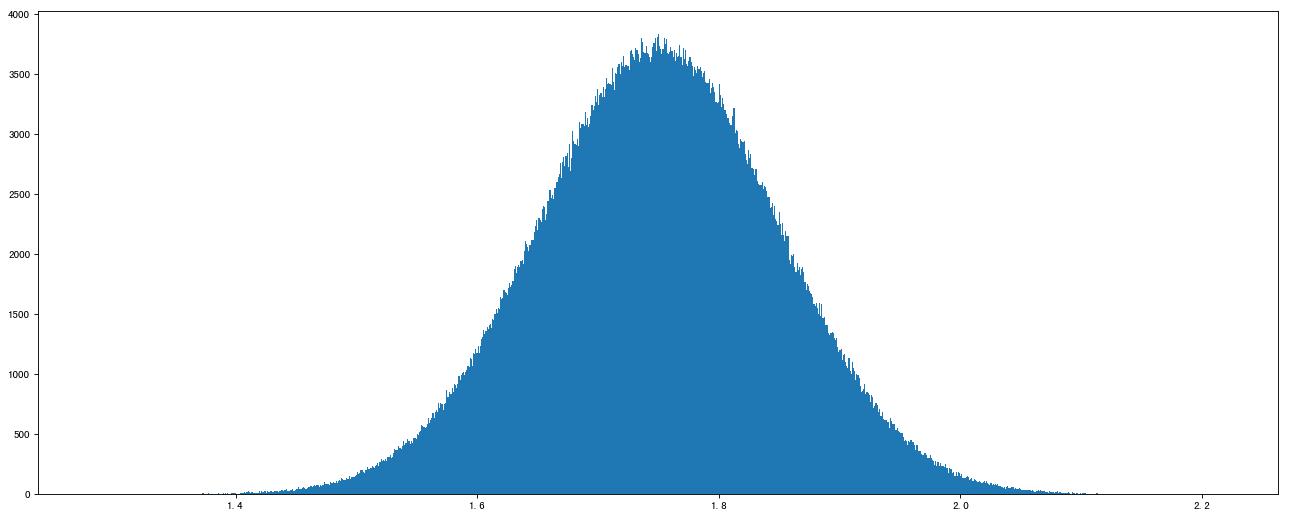
2.4、案例:随机生成8只股票2周的交易日涨幅数据
stock_change = np.random.normal(loc=0, scale=1, size=(8, 10))
stock_change
array([[-0.03469926, 1.68760014, 0.05915316, 2.4473136 , -0.61776756,
-0.56253866, -1.24738637, 0.48320978, 1.01227938, -1.44509723],
[-1.8391253 , -1.10142576, 0.09582268, 1.01589092, -1.20262068,
0.76134643, -0.76782097, -1.11192773, 0.81609586, 0.07659056],
[-0.74293074, -0.7836588 , 1.32639574, -0.52735663, 1.4167841 ,
2.10286726, -0.21687665, -0.33073563, -0.46648617, 0.07926839],
[ 0.45914676, -0.78330377, -1.10763289, 0.10612596, -0.63375855,
-1.88121415, 0.6523779 , -1.27459184, -0.1828502 , -0.76587891],
[-0.50413407, -1.35848099, -2.21633535, -1.39300681, 0.13159471,
0.65429138, 0.32207255, 1.41792558, 1.12357799, -0.68599018],
[ 0.3627785 , 1.00279706, -0.68137875, -2.14800075, -2.82895231,
-1.69360338, 1.43816168, -2.02116677, 1.30746801, 1.41979011],
[-2.93762047, 0.22199761, 0.98788788, 0.37899235, 0.28281886,
-1.75837237, -0.09262863, -0.92354076, 1.11467277, 0.76034531],
[-0.39473551, 0.28402164, -0.15729195, -0.59342945, -1.0311294 ,
-1.07651428, 0.18618331, 1.5780439 , 1.31285558, 0.10777784]])# 获取第一个股票的前3个交易日的涨跌幅数据
stock_change[0, :3]array([-0.03469926, 1.68760014, 0.05915316])
a1 = np.array([ [[1,2,3],[4,5,6]], [[12,3,34],[5,6,7]]])
a1 # (2, 2, 3)
array([[[ 1, 2, 3], [ 4, 5, 6]], [[12, 3, 34], [ 5, 6, 7]]])
a1.shape(2, 2, 3)
a1[1, 0, 2] = 100000
a1
array([[[ 1, 2, 3], [ 4, 5, 6]], [[ 12, 3, 100000], [ 5, 6, 7]]])
2.5、形状修改
# 需求:让刚才的股票行、日期列反过来,变成日期行,股票列
stock_change
array([[-0.03469926, 1.68760014, 0.05915316, 2.4473136 , -0.61776756, -0.56253866, -1.24738637, 0.48320978, 1.01227938, -1.44509723], [-1.8391253 , -1.10142576, 0.09582268, 1.01589092, -1.20262068, 0.76134643, -0.76782097, -1.11192773, 0.81609586, 0.07659056], [-0.74293074, -0.7836588 , 1.32639574, -0.52735663, 1.4167841 , 2.10286726, -0.21687665, -0.33073563, -0.46648617, 0.07926839], [ 0.45914676, -0.78330377, -1.10763289, 0.10612596, -0.63375855, -1.88121415, 0.6523779 , -1.27459184, -0.1828502 , -0.76587891], [-0.50413407, -1.35848099, -2.21633535, -1.39300681, 0.13159471, 0.65429138, 0.32207255, 1.41792558, 1.12357799, -0.68599018], [ 0.3627785 , 1.00279706, -0.68137875, -2.14800075, -2.82895231, -1.69360338, 1.43816168, -2.02116677, 1.30746801, 1.41979011], [-2.93762047, 0.22199761, 0.98788788, 0.37899235, 0.28281886, -1.75837237, -0.09262863, -0.92354076, 1.11467277, 0.76034531], [-0.39473551, 0.28402164, -0.15729195, -0.59342945, -1.0311294 , -1.07651428, 0.18618331, 1.5780439 , 1.31285558, 0.10777784]])
stock_change.reshape((10, 8))

stock_change.resize((10, 8))

stock_change.T
array([[-0.03469926, 1.68760014, 0.05915316, 2.4473136 , -0.61776756, -0.56253866, -1.24738637, 0.48320978], [ 1.01227938, -1.44509723, -1.8391253 , -1.10142576, 0.09582268, 1.01589092, -1.20262068, 0.76134643], [-0.76782097, -1.11192773, 0.81609586, 0.07659056, -0.74293074, -0.7836588 , 1.32639574, -0.52735663], [ 1.4167841 , 2.10286726, -0.21687665, -0.33073563, -0.46648617, 0.07926839, 0.45914676, -0.78330377], [-1.10763289, 0.10612596, -0.63375855, -1.88121415, 0.6523779 , -1.27459184, -0.1828502 , -0.76587891], [-0.50413407, -1.35848099, -2.21633535, -1.39300681, 0.13159471, 0.65429138, 0.32207255, 1.41792558], [ 1.12357799, -0.68599018, 0.3627785 , 1.00279706, -0.68137875, -2.14800075, -2.82895231, -1.69360338], [ 1.43816168, -2.02116677, 1.30746801, 1.41979011, -2.93762047, 0.22199761, 0.98788788, 0.37899235], [ 0.28281886, -1.75837237, -0.09262863, -0.92354076, 1.11467277, 0.76034531, -0.39473551, 0.28402164], [-0.15729195, -0.59342945, -1.0311294 , -1.07651428, 0.18618331, 1.5780439 , 1.31285558, 0.10777784]])
stock_change.astype("int32")array([[ 0, 1, 0, 2, 0, 0, -1, 0, 1, -1], [-1, -1, 0, 1, -1, 0, 0, -1, 0, 0], [ 0, 0, 1, 0, 1, 2, 0, 0, 0, 0], [ 0, 0, -1, 0, 0, -1, 0, -1, 0, 0], [ 0, -1, -2, -1, 0, 0, 0, 1, 1, 0], [ 0, 1, 0, -2, -2, -1, 1, -2, 1, 1], [-2, 0, 0, 0, 0, -1, 0, 0, 1, 0], [ 0, 0, 0, 0, -1, -1, 0, 1, 1, 0]], dtype=int32)
stock_change.tostring()b'\x95&\x99\xdd\x19\xc4\xa1\xbfm8\x88\x00i\x00\xfb?\x92\xbc\x81\xa1RI\xae?\xa2\x95x&\x19\x94\x03@\x9f?\xbev\xc0\xc4\xe3\xbf\x87\xf4H\x13Q\x00\xe2\xbf\x9eM\x85hK\xf5\xf3\xbf\x17mZ\xb2\xe8\xec\xde?U\xca\xd4\xdbK2\xf0?G\xc6\xbbD\x1e\x1f\xf7\xbf\x9f-\xb0\xa5\x0em\xfd\xbf\x9b\xd0h\x9dp\x9f\xf1\xbfyH\x8e\xc3\xd5\x87\xb8?\x1d\x89v\xd5\x16A\xf0?\x89Aj-\xef=\xf3\xbf\xbc\x8ea/\xf3\\\xe8?\x94\xb8\xbaJ\xfd\x91\xe8\xbfv\xc0\x92\xbct\xca\xf1\xbf\x82\x82\x19\x11u\x1d\xea?\xf2.\x96Qp\x9b\xb3?g\xed\xef\xb0\x16\xc6\xe7\xbf\xf2\xbf!\x9c\xbb\x13\xe9\xbf\x7fv\x1e\xbd\xea8\xf5?\x1e \x9d\x02\x1b\xe0\xe0\xbf?\x99O\xce%\xab\xf6?\x84;\xb9\x11\xac\xd2\x00@p\xe3\xa07\x9d\xc2\xcb\xbfop\x94\xc4\xc5*\xd5\xbfN\x15)\xca\xe8\xda\xdd\xbf4\xa8\x8b\xf1\xeeJ\xb4?Qd\x8e\x1c\xa9b\xdd?\xc8\x92\xb6\x10\xd3\x10\xe9\xbf\xf1\x80\x87C\xdd\xb8\xf1\xbf\x18\x02B \x12+\xbb?Xv\xb4\x02\xc0G\xe4\xbf\xa6,\x8a\x02t\x19\xfe\xbf\xb4\xc9\xaf\x9cG\xe0\xe4?wCsj\xbad\xf4\xbf\xbc\xb1\xd5\xa9\xa2g\xc7\xbf\xbc\xc6\x8d{\x14\x82\xe8\xbf>\xf7\xae\xc6\xdd!\xe0\xbf\xacB\x9c\x90V\xbc\xf5\xbfb\xae\xfa\x06\x0e\xbb\x01\xc0_B\xe1\x82\xc1I\xf6\xbfw\x9f\xb6m\x18\xd8\xc0?\x93\xcb\x8e{\xf4\xef\xe4?\xfe\xc1\xba,\xd6\x9c\xd4?k\x85)\xbc\xd2\xaf\xf6?{g\x82\xea,\xfa\xf1?s}\xaf\xad\xa1\xf3\xe5\xbfD(cM\xc37\xd7?(\x1a\xff\xect\x0b\xf0?7e\x80\xce\xda\xcd\xe5\xbf"\xd5\xe1\x03\x1b/\x01\xc0\x94\x85?\xbf\xb1\xa1\x06\xc0w\x08\x14\xdc\xff\x18\xfb\xbf\x9f\x1eL\xd2\xb5\x02\xf7?\xb0-5{Y+\x00\xc0;\xf5<\x94c\xeb\xf4?a\x8f\xb1\xd6u\xb7\xf6?%Kr)?\x80\x07\xc0\x9e\x1c%\xedjj\xcc?F\xa0C\t\xc7\x9c\xef?\xf3\xc3\xfd\x1eiA\xd8?\xcc\x9e\x84D\xb4\x19\xd2?\xdd$J\x10K"\xfc\xbf\xe6E\xb3\x95\x82\xb6\xb7\xbf\x0cN\xa4Z\xa5\x8d\xed\xbf\x96\xdd\xee\x1c\xb3\xd5\xf1?\x05\x8c\x12\xb0\xbfT\xe8?/\xa5\x1a\xb9XC\xd9\xbf~Z!\x1ci-\xd2?\x1f\xe4\xe3\x83$"\xc4\xbf_&\xc5\xc0_\xfd\xe2\xbf\xbf\x16\xac\x8b\x81\x7f\xf0\xbf\xf7\xba)\tg9\xf1\xbf\xb7q\x8c\xd7\xda\xd4\xc7?\x98P\xb7\xf4\xaa?\xf9?\x8c\x98P\xdbt\x01\xf5?t\xd8 -T\x97\xbb?'
3、数组的运算
3.1、数组去重
temp = np.array([[1, 2, 3, 4],[3, 4, 5, 6]])
temp
array([[1, 2, 3, 4], [3, 4, 5, 6]])
np.unique(temp)array([1, 2, 3, 4, 5, 6])
set(temp.flatten()), 2, 3, 4, 5, 6}
3.2、逻辑运算
stock_change = np.random.normal(loc=0, scale=1, size=(8, 10))

stock_change
array([[ 1.46338968, -0.45576704, 0.29667843, 0.16606916, 0.46446682, 0.83167611, -1.35770374, -0.65001192, 1.38319911, -0.93415832], [ 0.36775845, 0.24078108, 0.122042 , 1.19314047, 1.34072589, 0.09361683, 1.19030379, 1.4371421 , -0.97829363, -0.11962767], [-1.48252741, -0.69347186, 0.91122464, -0.30606473, 0.41598897, 0.79542753, -0.01447862, -1.49943117, -0.23285809, 0.42806777], [ 0.39438905, -1.31770556, 1.7344868 , -1.52812773, -0.47703227, -0.3795497 , -0.88422651, 1.37510973, -0.93622775, 0.49257673], [-0.9822216 , -1.09482936, -0.81834523, 0.57335311, 0.97390091, 0.05314952, -0.58316743, 0.19264426, 0.02081861, 0.84445247], [ 0.41739964, -0.26826893, -0.70003442, -0.58593912, 0.86546709, -1.30304864, 0.05254567, -1.73976785, -0.43532247, 0.4760526 ], [-0.21739882, 0.52007085, -0.60160491, 0.57108639, 1.03303301, -0.69172579, 1.04716985, -0.22985706, -0.11125069, 0.87722923], [-0.183266 , 0.56273065, 0.29357786, -0.19343363, -1.54547303, -0.31977163, -0.00659025, 0.48160678, 0.88443604, -0.48456825]])
# 逻辑判断, 如果涨跌幅大于0.5就标记为True 否则为False
stock_change > 0.5
array([[ True, False, False, False, False, True, False, False, True, False], [False, False, False, True, True, False, True, True, False, False], [False, False, True, False, False, True, False, False, False, False], [False, False, True, False, False, False, False, True, False, False], [False, False, False, True, True, False, False, False, False, True], [False, False, False, False, True, False, False, False, False, False], [False, True, False, True, True, False, True, False, False, True], [False, True, False, False, False, False, False, False, True, False]])
stock_change[stock_change > 0.5] = 1.1
stock_change
array([[ 1.1 , -0.45576704, 0.29667843, 0.16606916, 0.46446682, 1.1 , -1.35770374, -0.65001192, 1.1 , -0.93415832], [ 0.36775845, 0.24078108, 0.122042 , 1.1 , 1.1 , 0.09361683, 1.1 , 1.1 , -0.97829363, -0.11962767], [-1.48252741, -0.69347186, 1.1 , -0.30606473, 0.41598897, 1.1 , -0.01447862, -1.49943117, -0.23285809, 0.42806777], [ 0.39438905, -1.31770556, 1.1 , -1.52812773, -0.47703227, -0.3795497 , -0.88422651, 1.1 , -0.93622775, 0.49257673], [-0.9822216 , -1.09482936, -0.81834523, 1.1 , 1.1 , 0.05314952, -0.58316743, 0.19264426, 0.02081861, 1.1 ], [ 0.41739964, -0.26826893, -0.70003442, -0.58593912, 1.1 , -1.30304864, 0.05254567, -1.73976785, -0.43532247, 0.4760526 ], [-0.21739882, 1.1 , -0.60160491, 1.1 , 1.1 , -0.69172579, 1.1 , -0.22985706, -0.11125069, 1.1 ], [-0.183266 , 1.1 , 0.29357786, -0.19343363, -1.54547303, -0.31977163, -0.00659025, 0.48160678, 1.1 , -0.48456825]])
# 判断stock_change[0:2, 0:5]是否全是上涨的
stock_change[0:2, 0:5] > 0
array([[ True, False, True, True, True], [ True, True, True, True, True]])
np.all(stock_change[0:2, 0:5] > 0)False
# 判断前5只股票这段期间是否有上涨的
np.any(stock_change[:5, :] > 0)
True
3.3、np.where(三元运算符)
# 判断前四个股票前四天的涨跌幅 大于0的置为1,否则为0
temp = stock_change[:4, :4]
temp
array([[ 1.1 , -0.45576704, 0.29667843, 0.16606916], [ 0.36775845, 0.24078108, 0.122042 , 1.1 ], [-1.48252741, -0.69347186, 1.1 , -0.30606473], [ 0.39438905, -1.31770556, 1.1 , -1.52812773]])
np.where(temp > 0, 1, 0)array([[1, 0, 1, 1], [1, 1, 1, 1], [0, 0, 1, 0], [1, 0, 1, 0]])
temp > 0array([[ True, False, True, True], [ True, True, True, True], [False, False, True, False], [ True, False, True, False]])
np.where([[ True, False,  True,  True],
       [ True,  True,  True,  True],
       [False, False,  True, False],
       [ True, False,  True, False]], 1, 0)
array([[1, 0, 1, 1], [1, 1, 1, 1], [0, 0, 1, 0], [1, 0, 1, 0]])
temparray([[ 1.1 , -0.45576704, 0.29667843, 0.16606916], [ 0.36775845, 0.24078108, 0.122042 , 1.1 ], [-1.48252741, -0.69347186, 1.1 , -0.30606473], [ 0.39438905, -1.31770556, 1.1 , -1.52812773]])
# 判断前四个股票前四天的涨跌幅 大于0.5并且小于1的,换为1,否则为0
# (temp > 0.5) and (temp < 1)
np.logical_and(temp > 0.5, temp < 1)
array([[False, False, False, False], [False, False, False, False], [False, False, False, False], [False, False, False, False]])
# 判断前四个股票前四天的涨跌幅 大于0.5或者小于-0.5的,换为1,否则为0
np.logical_or(temp > 0.5, temp < -0.5)
array([[ True, False, False, False], [False, False, False, True], [ True, True, True, False], [False, True, True, True]])
np.where(np.logical_or(temp > 0.5, temp < -0.5), 11, 3)array([[11, 3, 3, 3], [ 3, 3, 3, 11], [11, 11, 11, 3], [ 3, 11, 11, 11]])
3.4、股票涨跌幅统计运算
# 前四只股票前四天的最大涨幅
temp
# shape: (4, 4) 0  1
array([[ 1.1 , -0.45576704, 0.29667843, 0.16606916], [ 0.36775845, 0.24078108, 0.122042 , 1.1 ], [-1.48252741, -0.69347186, 1.1 , -0.30606473], [ 0.39438905, -1.31770556, 1.1 , -1.52812773]])
temp.max(axis=0)array([1.1 , 0.24078108, 1.1 , 1.1 ])
np.max(temp, axis=-1)array([1.1, 1.1, 1.1, 1.1])
np.argmax(temp, axis=-1)array([0, 3, 2, 2])
3.5、数组与数的运算
arr = np.array([[1, 2, 3, 2, 1, 4], [5, 6, 1, 2, 3, 1]])
arr / 10
array([[0.1, 0.2, 0.3, 0.2, 0.1, 0.4], [0.5, 0.6, 0.1, 0.2, 0.3, 0.1]])
3.6、数组与数组的运算
arr1 = np.array([[1, 2, 3, 2, 1, 4], [5, 6, 1, 2, 3, 1]])
arr2 = np.array([[1, 2, 3, 4], [3, 4, 5, 6]])

arr1 # (2, 6)
array([[1, 2, 3, 2, 1, 4], [5, 6, 1, 2, 3, 1]])
arr2 # (2, 4)array([[1, 2, 3, 4], [3, 4, 5, 6]])
arr2 = np.array([[1], [3]])
arr2
array([[1], [3]])
arr1 + arr2array([[2, 3, 4, 3, 2, 5], [8, 9, 4, 5, 6, 4]])
arr1 * arr2array([[ 1, 2, 3, 2, 1, 4], [15, 18, 3, 6, 9, 3]])
arr1 / arr2array([[1. , 2. , 3. , 2. , 1. , 4. ], [1.66666667, 2. , 0.33333333, 0.66666667, 1. , 0.33333333]])
3.7、 矩阵运算
# ndarray存储矩阵
data = np.array([[80, 86],
[82, 80],
[85, 78],
[90, 90],
[86, 82],
[82, 90],
[78, 80],
[92, 94]])
# matrix存储矩阵
data_mat = np.mat([[80, 86],
[82, 80],
[85, 78],
[90, 90],
[86, 82],
[82, 90],
[78, 80],
[92, 94]])
type(data_mat)numpy.matrixlib.defmatrix.matrix
data # (8, 2) * (2, 1) = (8, 1)array([[80, 86], [82, 80], [85, 78], [90, 90], [86, 82], [82, 90], [78, 80], [92, 94]])
weights = np.array([[0.3], [0.7]])
weights
array([[0.3], [0.7]])
weights_mat = np.mat([[0.3], [0.7]])
weights_mat
matrix([[0.3], [0.7]])
np.matmul(data, weights)

data @ weights

np.dot(data, weights)

data_mat * weights_mat
array([[84.2], [80.6], [80.1], [90. ], [83.2], [87.6], [79.4], [93.4]])
3.8、 合并
a = stock_change[:2, 0:4]
b = stock_change[4:6, 0:4]
a
array([[ 1.1 , -0.45576704, 0.29667843, 0.16606916], [ 0.36775845, 0.24078108, 0.122042 , 1.1 ]])
a.shape(2, 4)
a.reshape((-1, 2))array([[ 1.1 , -0.45576704], [ 0.29667843, 0.16606916], [ 0.36775845, 0.24078108], [ 0.122042 , 1.1 ]])
barray([[-0.9822216 , -1.09482936, -0.81834523, 1.1 ], [ 0.41739964, -0.26826893, -0.70003442, -0.58593912]])
np.hstack((a, b))array([[ 1.1 , -0.45576704, 0.29667843, 0.16606916, -0.9822216 , -1.09482936, -0.81834523, 1.1 ], [ 0.36775845, 0.24078108, 0.122042 , 1.1 , 0.41739964, -0.26826893, -0.70003442, -0.58593912]])
np.concatenate((a, b), axis=1)array([[ 1.1 , -0.45576704, 0.29667843, 0.16606916, -0.9822216 , -1.09482936, -0.81834523, 1.1 ], [ 0.36775845, 0.24078108, 0.122042 , 1.1 , 0.41739964, -0.26826893, -0.70003442, -0.58593912]])
np.vstack((a, b))array([[ 1.1 , -0.45576704, 0.29667843, 0.16606916], [ 0.36775845, 0.24078108, 0.122042 , 1.1 ], [-0.9822216 , -1.09482936, -0.81834523, 1.1 ], [ 0.41739964, -0.26826893, -0.70003442, -0.58593912]])
np.concatenate((a, b), axis=0)array([[ 1.1 , -0.45576704, 0.29667843, 0.16606916], [ 0.36775845, 0.24078108, 0.122042 , 1.1 ], [-0.9822216 , -1.09482936, -0.81834523, 1.1 ], [ 0.41739964, -0.26826893, -0.70003442, -0.58593912]])
3.9、 Numpy读取
data = np.genfromtxt("test.csv", delimiter=",")
data
array([[ nan, nan, nan, nan], [ 1. , 123. , 1.4, 23. ], [ 2. , 110. , nan, 18. ], [ 3. , nan, 2.1, 19. ]])
type(data[2, 2])numpy.float64
def fill_nan_by_column_mean(t):
    for i in range(t.shape[1]):
        # 计算nan的个数
        nan_num = np.count_nonzero(t[:, i][t[:, i] != t[:, i]])
        if nan_num > 0:
            now_col = t[:, i]
            # 求和
            now_col_not_nan = now_col[np.isnan(now_col) == False].sum()
            # 和/个数
            now_col_mean = now_col_not_nan / (t.shape[0] - nan_num)
            # 赋值给now_col
            now_col[np.isnan(now_col)] = now_col_mean
            # 赋值给t,即更新t的当前列
            t[:, i] = now_col
return tdataarray([[ nan, nan, nan, nan], [ 1. , 123. , 1.4, 23. ], [ 2. , 110. , nan, 18. ], [ 3. , nan, 2.1, 19. ]])
fill_nan_by_column_mean(data)array([[ 2. , 116.5 , 1.75, 20. ], [ 1. , 123. , 1.4 , 23. ], [ 2. , 110. , 1.75, 18. ], [ 3. , 116.5 , 2.1 , 19. ]])
三、Pandas
什么是Pandas-数据处理工具
便捷的数据处理能力
集成了Numpy、Matplotlib
读取文件方便
import numpy as np
# 创建一个符合正态分布的10个股票5天的涨跌幅数据
stock_change = np.random.normal(0, 1, (10, 5))

stock_change
array([[-0.07726903, 0.40607587, 1.26740233, 1.48676212, -1.35987104], [ 0.28361364, 0.43101642, -0.77154311, 0.48286211, -0.30724683], [-0.98583786, -1.96339732, 0.31658224, -1.96541561, -0.39274454], [ 2.38020637, 1.47056011, -0.45253103, -0.77381961, 0.4822656 ], [ 2.05044671, -0.0743407 , 0.10900497, 0.00982431, -0.06639766], [-1.62883603, 2.370443 , -0.14230101, -1.73515932, 1.6128039 ], [ 0.59420384, 0.09903473, -2.82975368, 0.63599429, -0.40809638], [ 1.27884397, -0.42832722, 1.07118356, -0.04453698, -0.19217219], [ 0.35350472, -0.73933626, 0.81653138, -0.40873922, 1.24391025], [-0.66201232, -0.53088568, -2.01276069, 0.03709581, 0.86862061]])
0 |
1 |
2 |
3 |
4 |
|
0 |
-0.077269 |
0.406076 |
1.267402 |
1.486762 |
-1.359871 |
1 |
0.283614 |
0.431016 |
-0.771543 |
0.482862 |
-0.307247 |
2 |
-0.985838 |
-1.963397 |
0.316582 |
-1.965416 |
-0.392745 |
3 |
2.380206 |
1.470560 |
-0.452531 |
-0.773820 |
0.482266 |
4 |
2.050447 |
-0.074341 |
0.109005 |
0.009824 |
-0.066398 |
5 |
-1.628836 |
2.370443 |
-0.142301 |
-1.735159 |
1.612804 |
6 |
0.594204 |
0.099035 |
-2.829754 |
0.635994 |
-0.408096 |
7 |
1.278844 |
-0.428327 |
1.071184 |
-0.044537 |
-0.192172 |
8 |
0.353505 |
-0.739336 |
0.816531 |
-0.408739 |
1.243910 |
9 |
-0.662012 |
-0.530886 |
-2.012761 |
0.037096 |
0.868621 |
# 添加行索引
stock = ["股票{}".format(i) for i in range(10)]

pd.DataFrame(stock_change, index=stock)
0 |
1 |
2 |
3 |
4 |
|
股票0 |
-0.077269 |
0.406076 |
1.267402 |
1.486762 |
-1.359871 |
股票1 |
0.283614 |
0.431016 |
-0.771543 |
0.482862 |
-0.307247 |
股票2 |
-0.985838 |
-1.963397 |
0.316582 |
-1.965416 |
-0.392745 |
股票3 |
2.380206 |
1.470560 |
-0.452531 |
-0.773820 |
0.482266 |
股票4 |
2.050447 |
-0.074341 |
0.109005 |
0.009824 |
-0.066398 |
股票5 |
-1.628836 |
2.370443 |
-0.142301 |
-1.735159 |
1.612804 |
股票6 |
0.594204 |
0.099035 |
-2.829754 |
0.635994 |
-0.408096 |
股票7 |
1.278844 |
-0.428327 |
1.071184 |
-0.044537 |
-0.192172 |
股票8 |
0.353505 |
-0.739336 |
0.816531 |
-0.408739 |
1.243910 |
股票9 |
-0.662012 |
-0.530886 |
-2.012761 |
0.037096 |
0.868621 |
# 添加列索引
date = pd.date_range(start="20180101", periods=5, freq="B")
date
DatetimeIndex(['2018-01-01', '2018-01-02', '2018-01-03', '2018-01-04', '2018-01-05'], dtype='datetime64[ns]', freq='B')
data = pd.DataFrame(stock_change, index=stock, columns=date)
data
2018-01-01 00:00:00 |
2018-01-02 00:00:00 |
2018-01-03 00:00:00 |
2018-01-04 00:00:00 |
2018-01-05 00:00:00 |
|
股票0 |
-0.077269 |
0.406076 |
1.267402 |
1.486762 |
-1.359871 |
股票1 |
0.283614 |
0.431016 |
-0.771543 |
0.482862 |
-0.307247 |
股票2 |
-0.985838 |
-1.963397 |
0.316582 |
-1.965416 |
-0.392745 |
股票3 |
2.380206 |
1.470560 |
-0.452531 |
-0.773820 |
0.482266 |
股票4 |
2.050447 |
-0.074341 |
0.109005 |
0.009824 |
-0.066398 |
股票5 |
-1.628836 |
2.370443 |
-0.142301 |
-1.735159 |
1.612804 |
股票6 |
0.594204 |
0.099035 |
-2.829754 |
0.635994 |
-0.408096 |
股票7 |
1.278844 |
-0.428327 |
1.071184 |
-0.044537 |
-0.192172 |
股票8 |
0.353505 |
-0.739336 |
0.816531 |
-0.408739 |
1.243910 |
股票9 |
-0.662012 |
-0.530886 |
-2.012761 |
0.037096 |
0.868621 |