目录
引言
自2020年5月18日发布以来,已经经过过数个版本的迭代,当前最新版本为v7,添加了分割能力。已经有很多的博文讲解了yolov5的原理以及如何用标注的数据,比如YOLOv5网络详解 深入浅出Yolo系列之Yolov5核心基础知识完整讲解 手把手教你用深度学习做物体检测(一): 快速感受物体检测的酷炫
它的安装非常加单,使用方便,已经成为事实上的检测方法的基准
// 克隆代码库即可
git clone https://github.com/ultralytics/yolov5  # clone
cd yolov5
pip install -r requirements.txt  # install
使用时仅需要一行代码即可完成
import torch
# 加载模型
model = torch.hub.load('ultralytics/yolov5', 'yolov5s')  # or yolov5n - yolov5x6, custom
# 图片路径
img = 'https://ultralytics.com/images/zidane.jpg'  # or file, Path, PIL, OpenCV, numpy, list
# 执行检测推理
results = model(img)
# 检测结果可视化
results.print()  # or .show(), .save(), .crop(), .pandas(), etc.
什么?你一行代码也不想写,想无代码开发,直接从摄像头看效果,那直接运行仓库里的detect.py也能满足你的要求
python detect.py --weights yolov5s.pt --source 0详细参数含义如下,其中--weights指定你要使用的预训练权重,--source指定要检测的源(图片、图片路径列表、摄像头甚至是网络推流)
python detect.py --weights yolov5s.pt --source 0                               # webcam
                                               img.jpg                         # image
                                               vid.mp4                         # video
                                               screen                          # screenshot
                                               path/                           # directory
                                               list.txt                        # list of images
                                               list.streams                    # list of streams
                                               'path/*.jpg'                    # glob
                                               'https://youtu.be/Zgi9g1ksQHc'  # YouTube
                                               'rtsp://example.com/media.mp4'  # RTSP, RTMP, HTTP stream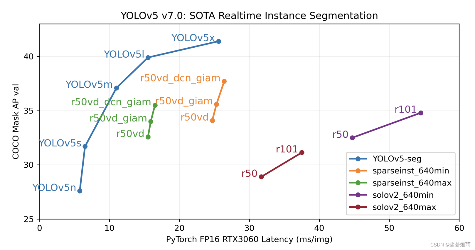
网络结构
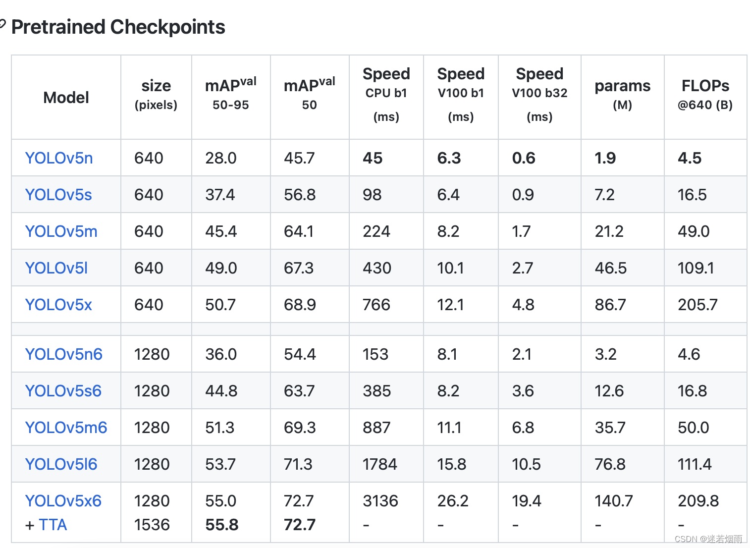
YOLOv5针对不同大小(n, s, m, l, x)的网络整体架构都是一样的,只不过会在每个子模块中采用不同的深度和宽度,分别应对yaml文件中的depth_multiple和width_multiple参数。还需要注意一点,官方除了n, s, m, l, x版本外还有n6, s6, m6, l6, x6,区别在于后者是针对更大分辨率的图片比如1280x1280,当然结构上也有些差异,后者会下采样64倍,采用4个预测特征层,而前者只会下采样到32倍且采用3个预测特征层。
YOLOv5在
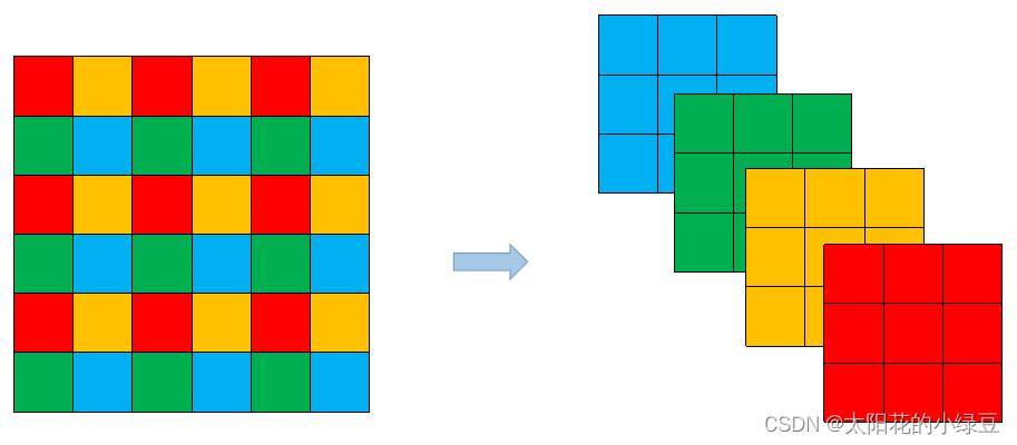
v6.0版本后相比之前版本有一个很小的改动,把网络的第一层(原来是Focus模块)换成了一个6x6大小的卷积层。两者在理论上其实等价的,但是对于现有的一些GPU设备(以及相应的优化算法)使用6x6大小的卷积层比使用Focus模块更加高效。详情可以参考这个issue #4825。下图是原来的Focus模块(和之前Swin Transformer中的Patch Merging类似),将每个2x2的相邻像素划分为一个patch,然后将每个patch中相同位置(同一颜色)像素给拼在一起就得到了4个feature map,然后在接上一个3x3大小的卷积层。这和直接使用一个6x6大小的卷积层等效。
Neck部分将
SPP换成成了SPPF(Glenn Jocher自己设计的),两者的作用是一样的,但后者效率更高。SPP结构是将输入并行通过多个不同大小的MaxPool,然后做进一步融合,能在一定程度上解决目标多尺度问题。而SPPF结构是将输入串行通过多个5x5大小的MaxPool层,这里需要注意的是串行两个5x5大小的MaxPool层是和一个9x9大小的MaxPool层计算结果是一样的,串行三个5x5大小的MaxPool层是和一个13x13大小的MaxPool层计算结果是一样的。

数据增强
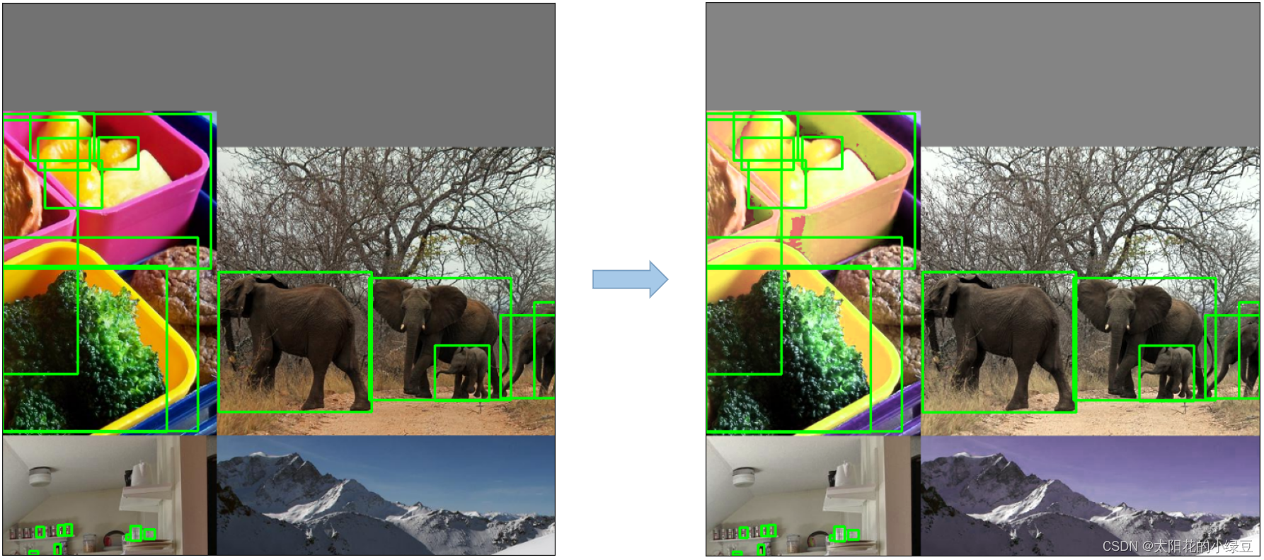
Mosaic,将四张图片拼成一张图片

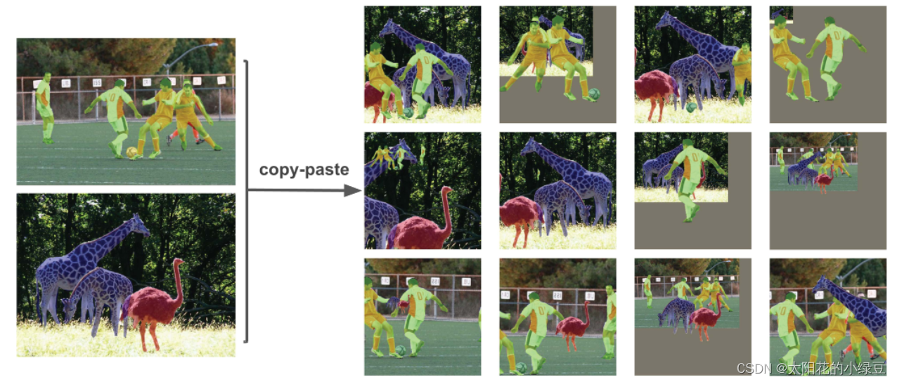
Copy paste,将部分目标随机的粘贴到图片中,前提是数据要有segments数据才行,即每个目标的实例分割信息
Random affine(Rotation, Scale, Translation and Shear),随机进行仿射变换,但根据配置文件里的超参数发现只使用了Scale和Translation即缩放和平移。

MixUp,就是将两张图片按照一定的透明度融合在一起,具体有没有用不太清楚,毕竟没有论文,也没有消融实验。代码中只有较大的模型才使用到了MixUp,而且每次只有10%的概率会使用到。

Albumentations,主要是做些滤波、直方图均衡化以及改变图片质量等等,我看代码里写的只有安装了albumentations包才会启用,但在项目的requirements.txt文件中albumentations包是被注释掉了的,所以默认不启用。
Augment HSV(Hue, Saturation, Value),随机调整色度,饱和度以及明度。
Random horizontal flip,随机水平翻转

在YOLOv5源码中使用到了很多训练的策略
- Multi-scale training(0.5~1.5x),多尺度训练,假设设置输入图片的大小为 640 × 640 ,训练时采用尺寸是在 0.5 × 640 ∼ 1.5 × 640之间随机取值,注意取值时取得都是32的整数倍(因为网络会最大下采样32倍)。
- AutoAnchor(For training custom data),训练自己数据集时可以根据自己数据集里的目标进行重新聚类生成Anchors模板。
- Warmup and Cosine LR scheduler,训练前先进行
Warmup热身,然后在采用Cosine学习率下降策略。- EMA(Exponential Moving Average),可以理解为给训练的参数加了一个动量,让它更新过程更加平滑。
- Mixed precision,混合精度训练,能够减少显存的占用并且加快训练速度,前提是GPU硬件支持。
- Evolve hyper-parameters,超参数优化,没有炼丹经验的人勿碰,保持默认就好。
YOLOv5的损失主要由三个部分组成:
- Classes loss,分类损失,采用的是
BCE loss,注意只计算正样本的分类损失。 - Objectness loss,
obj损失,采用的依然是BCE loss,注意这里的obj指的是网络预测的目标边界框与GT Box的CIoU。这里计算的是所有样本的obj损失。 - Location loss,定位损失,采用的是
CIoU loss,注意只计算正样本的定位损失。
部署
yolov5 v6.0(不含)之前的版本由于使用了Focus层,对部署造成了很大的不变,需要很多复杂的操作,详见详细记录u版YOLOv5目标检测ncnn实现, 具体修改步骤如下目标检测 YOLOv5 转ncnn移动端部署
// 1.导出onnx
python models/export.py --weights yolov5s.pt --img 320 --batch 1
// 2.简化模型
python -m onnxsim yolov5s.onnx yolov5s-sim.onnx
// 3. 模型转换到ncnn
./onnx2ncnn yolov5s-sim.onnx yolov5s.param yolov5s.bin
// 4. 编辑 yolov5s.param文件
第4行到13行删除(也就是Slice和Concat层),将第二行由172改成164(一共删除了10层,第二行的173更改为164,计算方法173-(10-1)=164)
增加自定义层
YoloV5Focus              focus                    1 1  images 159
其中159是刚才删除的Concat层的输出
// 5. 支持动态尺寸输入
将reshape中的960,240,60更改为-1,或者其他 0=后面的数
// 6. ncnnoptimize优化
./ncnnoptimize yolov5s.param yolov5s.bin yolov5s-opt.param yolov5s-opt.bin 1v6.0之后使用6x6的卷积代替,方便多了,可以直接使用opencv的dnn模块进行部署,详见Detecting objects with YOLOv5, OpenCV, Python and C++,代码yolov5-opencv-cpp-python
不过需要注意的是它只能配合opencv4.5.5及以上版本.主要包含6个步骤
// 1.加载模型
net = cv2.dnn.readNet('yolov5s.onnx')
// 2.加载图片
def format_yolov5(source):

    # put the image in square big enough
    col, row, _ = source.shape
    _max = max(col, row)
    resized = np.zeros((_max, _max, 3), np.uint8)
    resized[0:col, 0:row] = source

    # resize to 640x640, normalize to [0,1[ and swap Red and Blue channels
    result = cv2.dnn.blobFromImage(resized, 1/255.0, (640, 640), swapRB=True)

    return result
// 3.执行推理
predictions = net.forward()
output = predictions[0]
// 4.展开结果
def unwrap_detection(input_image, output_data):
    class_ids = []
    confidences = []
    boxes = []

    rows = output_data.shape[0]

    image_width, image_height, _ = input_image.shape

    x_factor = image_width / 640
    y_factor =  image_height / 640

    for r in range(rows):
        row = output_data[r]
        confidence = row[4]
        if confidence >= 0.4:

            classes_scores = row[5:]
            _, _, _, max_indx = cv2.minMaxLoc(classes_scores)
            class_id = max_indx[1]
            if (classes_scores[class_id] > .25):

                confidences.append(confidence)

                class_ids.append(class_id)

                x, y, w, h = row[0].item(), row[1].item(), row[2].item(), row[3].item()
                left = int((x - 0.5 * w) * x_factor)
                top = int((y - 0.5 * h) * y_factor)
                width = int(w * x_factor)
                height = int(h * y_factor)
                box = np.array([left, top, width, height])
                boxes.append(box)

// 5.非极大值抑制
indexes = cv2.dnn.NMSBoxes(boxes, confidences, 0.25, 0.45)

result_class_ids = []
result_confidences = []
result_boxes = []

for i in indexes:
    result_confidences.append(confidences[i])
    result_class_ids.append(class_ids[i])
    result_boxes.append(boxes[I])
// 6.可视化结果输出

class_list = []
with open("classes.txt", "r") as f:
    class_list = [cname.strip() for cname in f.readlines()]

colors = [(255, 255, 0), (0, 255, 0), (0, 255, 255), (255, 0, 0)]

for i in range(len(result_class_ids)):

    box = result_boxes[i]
    class_id = result_class_ids[i]

    color = colors[class_id % len(colors)]

    conf  = result_confidences[i]

    cv2.rectangle(image, box, color, 2)
    cv2.rectangle(image, (box[0], box[1] - 20), (box[0] + box[2], box[1]), color, -1)
    cv2.putText(image, class_list[class_id], (box[0] + 5, box[1] - 5), cv2.FONT_HERSHEY_SIMPLEX, 0.5, (0,0,0))
生成数据进行圆形和矩形检测
接下来以一个检测圆形和矩形的项目展示了yolov5的训练数据生成以及训练流程。但是标注数据是一项费时费力的工作,如果能用生成的数据来快速验证一些实验,岂不美哉。
基于Lable Studio【yoloV5实战记录】小白也能训练自己的数据集!基于labelimg 手把手教你用深度学习做物体检测(二):数据标注 - 程序员
yolov5的的标注格式非常简单,图片放置于images文件夹下,在labeles文件夹下每个图片文件都有一个同名对应的txt文件,里面按行保存每个目标的类别、归一化坐标和宽高,很多标注工具都支持直接导出yolo的标注格式,也有很多脚本可以很轻松的完成从VOC、coco等格式到YOLO格式的转换.
类别1 归一化中心点坐标x 归一化中心坐标y 归一化宽度 归一化高度
类别2 归一化中心点坐标x 归一化中心坐标y 归一化宽度 归一化高度
1. 这里以检测圆为例,详细介绍每个步骤
首先是训练数据的生成和可视化, 随机的以某点为圆心,以60-100为半径画一个颜色随机的圆作为我们要检测的目标,总共生成10万张训练数据
import os
import cv2
import math
import random
import numpy as np
from tqdm import tqdm

def generate():
    img = np.zeros((640,640,3),np.uint8)
    x = 100+random.randint(0, 400)
    y = 100+random.randint(0, 400)
    radius = random.randint(60,100)
    r = random.randint(0,255)
    g = random.randint(0,255)
    b = random.randint(0,255)
    cv2.circle(img, (x,y), radius, (b,g,r),-1)
    return img, [x,y,radius]

def generate_batch(num=10000):
    images_dir = "data/circle/images"
    if not os.path.exists(images_dir):
        os.makedirs(images_dir)
    labels_dir = "data/circle/labels"
    if not os.path.exists(labels_dir):
            os.makedirs(labels_dir)
    for i in tqdm(range(num)):
        img, labels = generate()
        cv2.imwrite(images_dir+"/"+str(i)+".jpg", img)
        with open(labels_dir+"/"+str(i)+".txt", 'w') as f:
            x, y, radius = labels
            f.write("0 "+str(x/640)+" "+str(y/640)+" "+str(2*radius/640)+" "+str(2*radius/640)+"\n")

def show_gt(dir='data/circle'):
    files = os.listdir(dir+"/images")
    gtdir = dir+"/gt"
    if not os.path.exists(gtdir):
        os.makedirs(gtdir)
    for file in tqdm(files):
        imgpath = dir+"/images/"+file
        img = cv2.imread(imgpath)
        h,w,_ = img.shape
        labelpath = dir+"/labels/"+file[:-3]+"txt"
        with open(labelpath) as f:
            lines = f.readlines()
            for line in lines:
                items = line[:-1].split(" ")
                c = int(items[0])
                cx = float(items[1])
                cy = float(items[2])
                cw = float(items[3])
                ch = float(items[4])
                x1 = int((cx - cw/2)*w)
                y1 = int((cy - ch/2)*h)
                x2 = int((cx + cw/2)*w)
                y2 = int((cy + ch/2)*h)
                cv2.rectangle(img, (x1,y1),(x2,y2),(0,255,0),2)
            cv2.imwrite(gtdir+"/"+file, img)

if __name__=="__main__":
    generate_batch()
    show_gt()

然后构造circle.yaml
train: data/circle/images/
val: data/circle/images/
# number of classes
nc: 1

# class names
names: ['circle']
2.如果要检测圆形和长方形两类目标,则需要调整生成脚本和数据配置文件
import os
import cv2
import math
import random
import numpy as np
from tqdm import tqdm

def generate_circle():
    img = np.zeros((640,640,3),np.uint8)
    x = 100+random.randint(0, 400)
    y = 100+random.randint(0, 400)
    radius = random.randint(60,100)
    r = random.randint(0,255)
    g = random.randint(0,255)
    b = random.randint(0,255)
    cv2.circle(img, (x,y), radius, (b,g,r),-1)
    return img, [x,y,radius*2,radius*2]

def generate_rectangle():
    img = np.zeros((640,640,3),np.uint8)
    x1 = 100+random.randint(0, 400)
    y1 = 100+random.randint(0, 400)
    w = random.randint(80, 200)
    h = random.randint(80, 200)
    x2 = x1 + w
    y2 = y1 + h
    r = random.randint(0,255)
    g = random.randint(0,255)
    b = random.randint(0,255)
    cx = (x1+x2)//2
    cy = (y1+y2)//2
    cv2.rectangle(img, (x1,y1), (x2,y2), (b,g,r),-1)
    return img, [cx,cy,w,h]

def generate_batch(num=100000):
    images_dir = "data/shape/images"
    if not os.path.exists(images_dir):
        os.makedirs(images_dir)
    labels_dir = "data/shape/labels"
    if not os.path.exists(labels_dir):
            os.makedirs(labels_dir)
    for i in tqdm(range(num)):
        if i % 2 == 0:
            img, labels = generate_circle()
        else:
            img, labels = generate_rectangle()
        cv2.imwrite(images_dir+"/"+str(i)+".jpg", img)
        with open("data/shape/labels/"+str(i)+".txt", 'w') as f:
            cx,cy,w,h = labels
            f.write(str(i%2)+" "+str(cx/640)+" "+str(cy/640)+" "+str(w/640)+" "+str(h/640)+"\n")

def show_gt(dir='data/shape'):
    files = os.listdir(dir+"/images")
    gtdir = dir+"/gt"
    if not os.path.exists(gtdir):
        os.makedirs(gtdir)
    for file in tqdm(files):
        imgpath = dir+"/images/"+file
        img = cv2.imread(imgpath)
        h, w, _ = img.shape
        labelpath = dir+"/labels/"+file[:-3]+"txt"
        with open(labelpath) as f:
            lines = f.readlines()
            for line in lines:
                items = line[:-1].split(" ")
                c = int(items[0])
                cx = float(items[1])
                cy = float(items[2])
                cw = float(items[3])
                ch = float(items[4])
                x1 = int((cx - cw/2)*w)
                y1 = int((cy - ch/2)*h)
                x2 = int((cx + cw/2)*w)
                y2 = int((cy + ch/2)*h)
                cv2.rectangle(img, (x1,y1),(x2,y2),(0,255,0),2)
                cv2.putText(img, str(c), (x1,y1), 3,1,(0,0,255))
            cv2.imwrite(gtdir+"/"+file, img)

if __name__=="__main__":
    generate_batch()
    show_gt()
对应的shape.yaml, 注意类别数是2
train: data/shape/images/
val: data/shape/images/
# number of classes
nc: 2

# class names
names: ['circle', 'rectangle']
训练
使用如下命令启动训练
python train.py --data circle.yaml --cfg yolov5s.yaml --weights '' --batch-size 64如果是圆形和长方形两类目标, 命令为
python train.py --data shape.yaml --cfg yolov5s.yaml --weights '' --batch-size 64


看下训练过程中打印的统计信息,类别和分布情况

训几个epoch看下结果
               epoch,      train/box_loss,      train/obj_loss,      train/cls_loss,   metrics/precision,      metrics/recall,     metrics/mAP_0.5,metrics/mAP_0.5:0.95,        val/box_loss,        val/obj_loss,        val/cls_loss,               x/lr0,               x/lr1,               x/lr2
                   0,             0.03892,            0.011817,                   0,             0.99998,             0.99978,               0.995,             0.92987,           0.0077891,           0.0030948,                   0,           0.0033312,           0.0033312,            0.070019
                   1,            0.017302,           0.0049876,                   0,                   1,              0.9999,               0.995,             0.99105,           0.0031843,           0.0015662,                   0,           0.0066644,           0.0066644,            0.040019
                   2,            0.011272,           0.0034826,                   0,                   1,             0.99994,               0.995,             0.99499,           0.0020194,           0.0010969,                   0,           0.0099969,           0.0099969,            0.010018
                   3,           0.0080153,           0.0027186,                   0,                   1,             0.99994,               0.995,               0.995,           0.0013095,          0.00083033,                   0,           0.0099978,           0.0099978,           0.0099978
                   4,           0.0067639,           0.0023831,                   0,                   1,             0.99996,               0.995,               0.995,          0.00099513,          0.00068878,                   0,           0.0099978,           0.0099978,           0.0099978
                   5,           0.0061637,           0.0022279,                   0,                   1,             0.99996,               0.995,               0.995,          0.00090497,          0.00064193,                   0,           0.0099961,           0.0099961,           0.0099961
                   6,           0.0058844,            0.002144,                   0,             0.99999,             0.99998,               0.995,               0.995,           0.0009117,          0.00063328,                   0,           0.0099938,           0.0099938,           0.0099938
                   7,           0.0056247,             0.00208,                   0,             0.99999,             0.99999,               0.995,               0.995,          0.00086355,          0.00061343,                   0,           0.0099911,           0.0099911,           0.0099911
                   8,           0.0054567,           0.0020223,                   0,                   1,             0.99999,               0.995,               0.995,          0.00081632,          0.00059592,                   0,           0.0099879,           0.0099879,           0.0099879
                   9,           0.0053597,           0.0019864,                   0,                   1,                   1,               0.995,               0.995,          0.00081379,          0.00058942,                   0,           0.0099842,           0.0099842,           0.0099842
                  10,           0.0053103,           0.0019559,                   0,                   1,                   1,               0.995,               0.995,           0.0008175,          0.00058669,                   0,             0.00998,             0.00998,             0.00998
                  11,           0.0052146,           0.0019445,                   0,                   1,                   1,               0.995,               0.995,          0.00083248,          0.00058731,                   0,           0.0099753,           0.0099753,           0.0099753
                  12,           0.0050852,           0.0019065,                   0,                   1,                   1,               0.995,               0.995,          0.00085092,          0.00058853,                   0,           0.0099702,           0.0099702,           0.0099702
                  13,           0.0050589,           0.0019031,                   0,                   1,                   1,               0.995,               0.995,          0.00086915,          0.00059267,                   0,           0.0099645,           0.0099645,           0.0099645
                  14,           0.0049664,           0.0018693,                   0,                   1,                   1,               0.995,               0.995,          0.00090856,          0.00059815,                   0,           0.0099584,           0.0099584,           0.0099584
                  15,           0.0049839,           0.0018568,                   0,                   1,                   1,               0.995,               0.995,          0.00093147,          0.00060425,                   0,           0.0099517,           0.0099517,           0.0099517
                  16,           0.0049079,           0.0018459,                   0,                   1,                   1,               0.995,               0.995,           0.0009656,          0.00061124,                   0,           0.0099446,           0.0099446,           0.0099446
                  17,           0.0048693,           0.0018277,                   0,                   1,                   1,               0.995,               0.995,          0.00099703,          0.00061948,                   0,            0.009937,            0.009937,            0.009937
                  18,           0.0048052,           0.0018103,                   0,                   1,                   1,               0.995,               0.995,           0.0010246,          0.00062618,                   0,           0.0099289,           0.0099289,           0.0099289
                  19,           0.0047608,           0.0017947,                   0,                   1,                   1,               0.995,               0.995,           0.0010439,          0.00063123,                   0,           0.0099203,           0.0099203,           0.0099203
mAP达到99.5+,真不错,看下预测结果


圆形和长方形两类物体的


部署
最后使用如下命令进行检测,记得路径换成本地的路径
python detect.py --weights exps/yolov5s_circle/weights/best.pt --source data/circle/images 

自带的demo为了兼容各种格式太过啰嗦,转成onnx部署代码要简洁很多
import cv2
import numpy as np
import torch
from torchvision import transforms
import onnxruntime
from utils.general import non_max_suppression

def detect(img, ort_session):
    img = img.astype(np.float32)
    img = img / 255
    img_tensor = img.transpose(2,0,1)[None]
    ort_inputs = {ort_session.get_inputs()[0].name: img_tensor}
    pred = torch.tensor(ort_session.run(None, ort_inputs)[0])
    dets = non_max_suppression(pred, 0.25, 0.45)
    return dets[0]

def demo():
    ort_session = onnxruntime.InferenceSession("yolov5s.onnx",  providers=['TensorrtExecutionProvider'])
    img = cv2.imread("data/images/bus.jpg")
    img = cv2.resize(img,(640,640))
    dets = detect(img, ort_session)
    for det in dets:
        x1 = int(det[0])
        y1 = int(det[1])
        x2 = int(det[2])
        y2 = int(det[3])
        score = float(det[4])
        cls = int(det[5])
        info = "{}_{:.2f}".format(cls, score*100)
        cv2.rectangle(img, (x1,y1),(x2,y2),(255,255,0))
        cv2.putText(img, info, (x1,y1), 1, 1, (0,0,255))
    cv2.imwrite("runs/detect/bus.jpg", img)
if __name__=="__main__":
    demo()
总结
本文通过圆形检测和长方形检测两个例子详细讲解了如何生成训练数据所需的标签,并且给出了训练、测试和部署等全流程的代码实现