在之前的教程 “Elasticsearch:pipeline aggregation 介绍 (一)” 中,我们讨论了 Elasticsearch 管道聚合的结构,并指导你设置了几个常见的管道,例如导数、累积和和平均桶聚合。
在本文中,我们将继续分析 Elasticsearch 管道聚合,重点关注统计(stats)、移动平均(moving averages)和移动函数(moving functions)、百分位数(percentiles)、桶排序和桶脚本等管道。 Kibana 支持本文中讨论的一些管道聚合,例如移动平均线,因此我们还将向你展示如何将它们可视化。 让我们开始吧!
准备数据
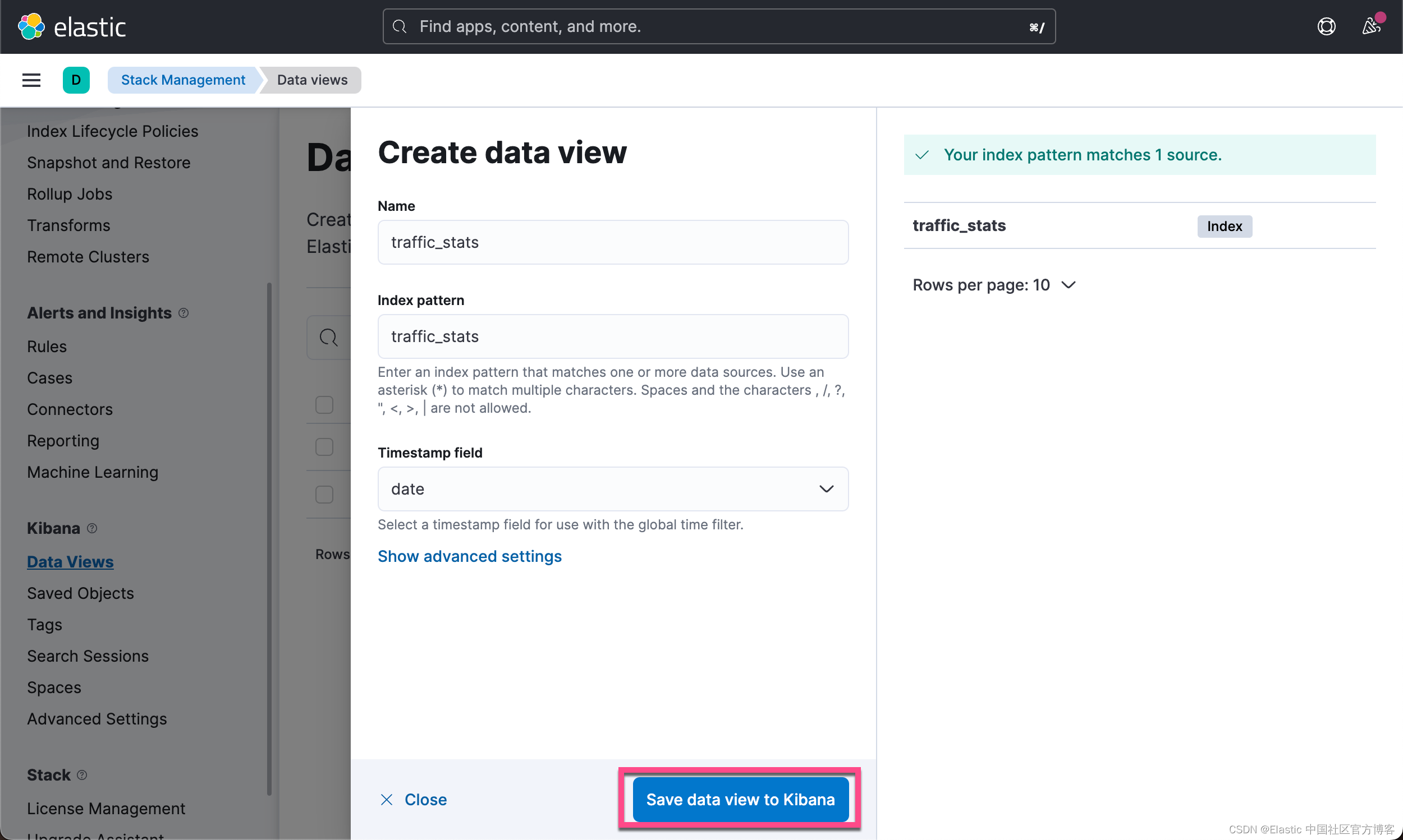
我们在 Kibana 中打入如下的命令来创建一个叫做 traffic_stats 的索引:
PUT traffic_stats
{
  "mappings": {
    "properties": {
      "date": {
        "type": "date",
        "format": "dateOptionalTime"
      },
      "visits": {
        "type": "integer"
      },
      "max_time_spent": {
        "type": "integer"
      }
    }
  }
}
由于一些原因,在最新的版本,比如 8.6.x 版本中,上述的命令可能不成功,你需要使用如下的格式来运行:
PUT traffic_stats
{
  "mappings": {
    "properties": {
      "date": {
        "type": "date",
        "format": "date_optional_time"
      },
      "visits": {
        "type": "integer"
      },
      "max_time_spent": {
        "type": "integer"
      }
    }
  }
}
创建索引映射后,让我们向其中保存一些任意数据:
PUT _bulk
{"index":{"_index":"traffic_stats"}}
{"visits":"488", "date":"2018-10-1", "max_time_spent":"900"}
{"index":{"_index":"traffic_stats"}}
{"visits":"783", "date":"2018-10-6", "max_time_spent":"928"}
{"index":{"_index":"traffic_stats"}}
{"visits":"789", "date":"2018-10-12", "max_time_spent":"1834"}
{"index":{"_index":"traffic_stats"}}
{"visits":"1299", "date":"2018-11-3", "max_time_spent":"592"}
{"index":{"_index":"traffic_stats"}}
{"visits":"394", "date":"2018-11-6", "max_time_spent":"1249"}
{"index":{"_index":"traffic_stats"}}
{"visits":"448", "date":"2018-11-24", "max_time_spent":"874"}
{"index":{"_index":"traffic_stats"}}
{"visits":"768", "date":"2018-12-18", "max_time_spent":"876"}
{"index":{"_index":"traffic_stats"}}
{"visits":"1194", "date":"2018-12-24", "max_time_spent":"1249"}
{"index":{"_index":"traffic_stats"}}
{"visits":"987", "date":"2018-12-28", "max_time_spent":"1599"}
{"index":{"_index":"traffic_stats"}}
{"visits":"872", "date":"2019-01-1", "max_time_spent":"828"}
{"index":{"_index":"traffic_stats"}}
{"visits":"972", "date":"2019-01-5", "max_time_spent":"723"}
{"index":{"_index":"traffic_stats"}}
{"visits":"827", "date":"2019-02-5", "max_time_spent":"1300"}
{"index":{"_index":"traffic_stats"}}
{"visits":"1584", "date":"2019-02-15", "max_time_spent":"1500"}
{"index":{"_index":"traffic_stats"}}
{"visits":"1604", "date":"2019-03-2", "max_time_spent":"1488"}
{"index":{"_index":"traffic_stats"}}
{"visits":"1499", "date":"2019-03-27", "max_time_spent":"1399"}
{"index":{"_index":"traffic_stats"}}
{"visits":"1392", "date":"2019-04-8", "max_time_spent":"1294"}
{"index":{"_index":"traffic_stats"}}
{"visits":"1247", "date":"2019-04-15", "max_time_spent":"1194"}
{"index":{"_index":"traffic_stats"}}
{"visits":"984", "date":"2019-05-15", "max_time_spent":"1184"}
{"index":{"_index":"traffic_stats"}}
{"visits":"1228", "date":"2019-05-18", "max_time_spent":"1485"}
{"index":{"_index":"traffic_stats"}}
{"visits":"1423", "date":"2019-06-14", "max_time_spent":"1452"}
{"index":{"_index":"traffic_stats"}}
{"visits":"1238", "date":"2019-06-24", "max_time_spent":"1329"}
{"index":{"_index":"traffic_stats"}}
{"visits":"1388", "date":"2019-07-14", "max_time_spent":"1542"}
{"index":{"_index":"traffic_stats"}}
{"visits":"1499", "date":"2019-07-24", "max_time_spent":"1742"}
{"index":{"_index":"traffic_stats"}}
{"visits":"1523", "date":"2019-08-13", "max_time_spent":"1552"}
{"index":{"_index":"traffic_stats"}}
{"visits":"1443", "date":"2019-08-19", "max_time_spent":"1511"}
{"index":{"_index":"traffic_stats"}}
{"visits":"1587", "date":"2019-09-14", "max_time_spent":"1497"}
{"index":{"_index":"traffic_stats"}}
{"visits":"1534", "date":"2019-09-27", "max_time_spent":"1434"}
太棒了! 现在,一切都已准备就绪,可以说明一些管道聚合。 让我们从统计桶聚合开始。为了下面可视化的需求,你需要在 Kibana 中为这个 traffic_stats 创建 index pattern (早期版本)或者 Data view:

Stats Bucket Aggregation
Stats 聚合计算一组统计指标,例如索引中某些数字字段的最小值(min)、最大值(Max)、平均值(avg)和总和(sum)。在 Elasticsearch 中,还可以计算由其他聚合生成的桶的统计数据。 当 stats 聚合所需的值必须首先使用其他聚合按桶计算时,这非常有用。
为了理解这个想法,让我们看一下下面的例子:
GET traffic_stats/_search?filter_path=aggregations
{
  "size": 0,
  "aggs": {
    "visits_per_month": {
      "date_histogram": {
        "field": "date",
        "calendar_interval": "month"
      },
      "aggs": {
        "total_visits": {
          "sum": {
            "field": "visits"
          }
        }
      }
    },
    "stats_monthly_visits": {
      "stats_bucket": {
        "buckets_path": "visits_per_month>total_visits"
      }
    }
  }
}
在此查询中,我们首先为 “visits” 字段生成一个日期直方图,并计算每个生成的桶的每月总访问量。 接下来,我们使用 stats 管道为每个生成的桶计算统计数据。 响应应如下所示:
{
  "aggregations": {
    "visits_per_month": {
      "buckets": [
        {
          "key_as_string": "2018-10-01T00:00:00.000Z",
          "key": 1538352000000,
          "doc_count": 3,
          "total_visits": {
            "value": 2060
          }
        },
        {
          "key_as_string": "2018-11-01T00:00:00.000Z",
          "key": 1541030400000,
          "doc_count": 3,
          "total_visits": {
            "value": 2141
          }
        },
        {
          "key_as_string": "2018-12-01T00:00:00.000Z",
          "key": 1543622400000,
          "doc_count": 3,
          "total_visits": {
            "value": 2949
          }
        },
        {
          "key_as_string": "2019-01-01T00:00:00.000Z",
          "key": 1546300800000,
          "doc_count": 2,
          "total_visits": {
            "value": 1844
          }
        },
        {
          "key_as_string": "2019-02-01T00:00:00.000Z",
          "key": 1548979200000,
          "doc_count": 2,
          "total_visits": {
            "value": 2411
          }
        },
        {
          "key_as_string": "2019-03-01T00:00:00.000Z",
          "key": 1551398400000,
          "doc_count": 2,
          "total_visits": {
            "value": 3103
          }
        },
        {
          "key_as_string": "2019-04-01T00:00:00.000Z",
          "key": 1554076800000,
          "doc_count": 2,
          "total_visits": {
            "value": 2639
          }
        },
        {
          "key_as_string": "2019-05-01T00:00:00.000Z",
          "key": 1556668800000,
          "doc_count": 2,
          "total_visits": {
            "value": 2212
          }
        },
        {
          "key_as_string": "2019-06-01T00:00:00.000Z",
          "key": 1559347200000,
          "doc_count": 2,
          "total_visits": {
            "value": 2661
          }
        },
        {
          "key_as_string": "2019-07-01T00:00:00.000Z",
          "key": 1561939200000,
          "doc_count": 2,
          "total_visits": {
            "value": 2887
          }
        },
        {
          "key_as_string": "2019-08-01T00:00:00.000Z",
          "key": 1564617600000,
          "doc_count": 2,
          "total_visits": {
            "value": 2966
          }
        },
        {
          "key_as_string": "2019-09-01T00:00:00.000Z",
          "key": 1567296000000,
          "doc_count": 2,
          "total_visits": {
            "value": 3121
          }
        }
      ]
    },
    "stats_monthly_visits": {
      "count": 12,
      "min": 1844,
      "max": 3121,
      "avg": 2582.8333333333335,
      "sum": 30994
    }
  }
}
在后台,stats 聚合对日期直方图生成的桶执行最小、最大、平均和求和管道聚合,计算结果,然后在响应结束时反映它们。
扩展统计(extended stats)桶聚合具有相同的逻辑,只是它返回额外的统计信息,如方差、平方和、标准差和标准差界限。 让我们稍微调整上面的查询以使用扩展的统计管道:
GET traffic_stats/_search?filter_path=aggregations
{
  "size": 0,
  "aggs": {
    "visits_per_month": {
      "date_histogram": {
        "field": "date",
        "calendar_interval": "month"
      },
      "aggs": {
        "total_visits": {
          "sum": {
            "field": "visits"
          }
        }
      }
    },
    "stats_monthly_visits": {
      "extended_stats_bucket": {
        "buckets_path": "visits_per_month>total_visits"
      }
    }
  }
}
响应将包含比简单的统计桶聚合更多的统计信息:
"stats_monthly_visits": {
"count": 12,
"min": 1844,
"max": 3121,
"avg": 2582.8333333333335,
"sum": 30994,
"sum_of_squares": 82176700,
"variance": 177030.30555555597,
"variance_population": 177030.30555555597,
"variance_sampling": 193123.96969697016,
"std_deviation": 420.7496946588981,
"std_deviation_population": 420.7496946588981,
"std_deviation_sampling": 439.4587235417795,
"std_deviation_bounds": {
"upper": 3424.3327226511296,
"lower": 1741.3339440155373,
"upper_population": 3424.3327226511296,
"lower_population": 1741.3339440155373,
"upper_sampling": 3461.7507804168927,
"lower_sampling": 1703.9158862497745
}
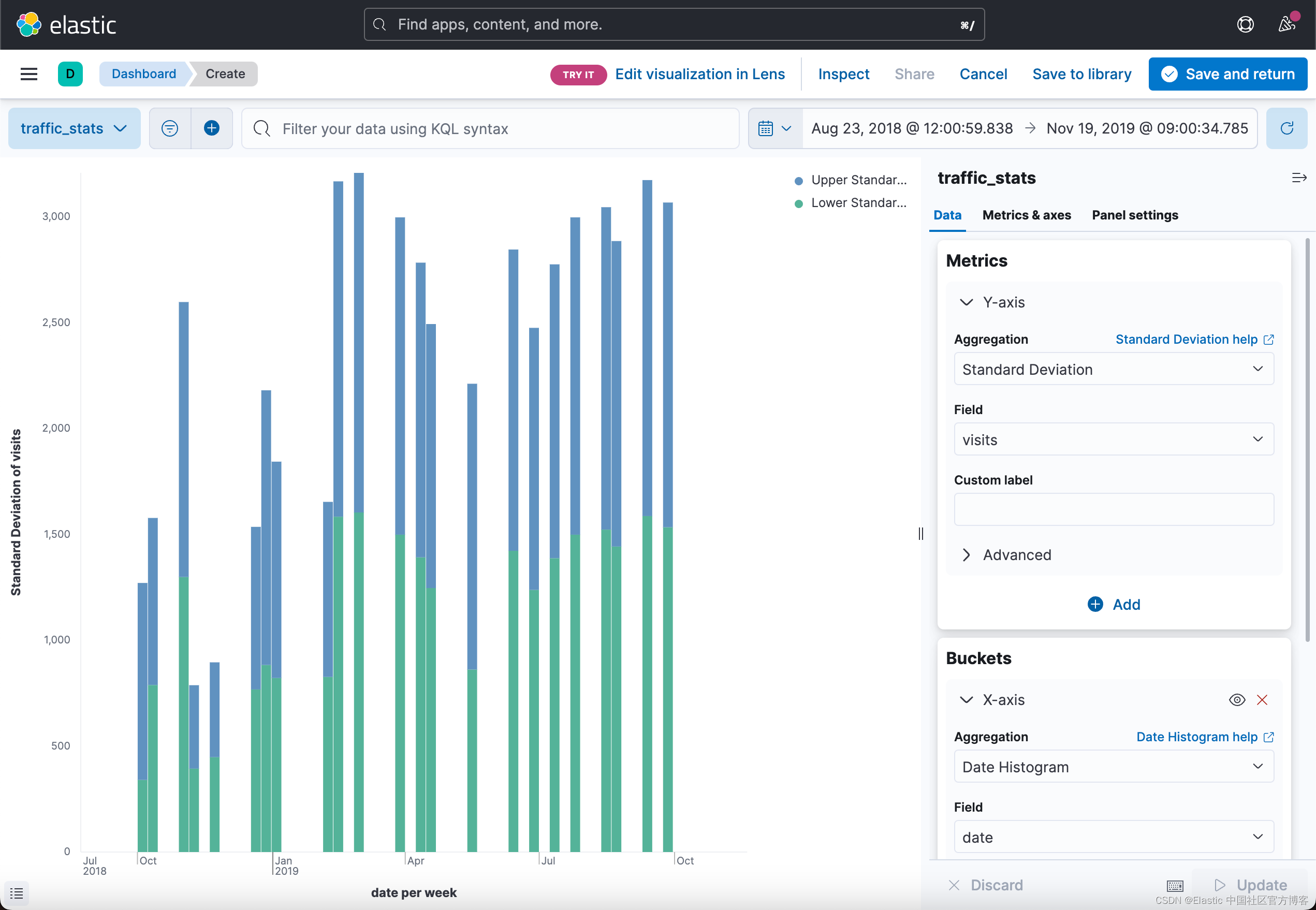
}Kibana 支持标准偏差边界的可视化,你可能会在上面的响应中看到这一点。 在下图中,我们看到日期直方图生成的每个桶的标准差上限(蓝色)和标准差下限(绿色):
Percentiles Bucket Aggregation
你还记得,百分位数(percentile)是一种统计量度,表示组中给定百分比的观察值低于该值的值。 例如,第 65 个百分位数是低于该值的 65% 的观测值。
一个简单的百分位数度量聚合计算索引数据中直接可用的值的百分位数。 但是,在某些情况下,你想要使用日期直方图生成存储桶并在应用百分位数之前计算这些存储桶的值。
当我们可以使用适用于父(parent)聚合生成的桶和兄弟(sibling)聚合计算的一些指标的百分位数桶管道时,情况就是如此。 看看下面的例子:
GET traffic_stats/_search?filter_path=aggregations
{
  "aggs": {
    "visits_per_month": {
      "date_histogram": {
        "field": "date",
        "calendar_interval": "month"
      },
      "aggs": {
        "total_visits": {
          "sum": {
            "field": "visits"
          }
        }
      }
    },
    "percentiles_monthly_visits": {
      "percentiles_bucket": {
        "buckets_path": "visits_per_month>total_visits",
        "percents": [
          15,
          50,
          75,
          99
        ]
      }
    }
  }
}
在这里,我们为日期直方图生成的每个存储桶中的 total_visits 指标的输出计算百分位数。 与常规百分位数聚合类似,百分位数管道聚合允许指定要返回的一组百分位数。 在这种情况下,我们选择计算第 15、50、75 和 99 个百分位数,这反映在聚合的百分比字段中。
上面的查询应该返回以下响应:
{
  "aggregations": {
    "visits_per_month": {
      "buckets": [
        {
          "key_as_string": "2018-10-01T00:00:00.000Z",
          "key": 1538352000000,
          "doc_count": 3,
          "total_visits": {
            "value": 2060
          }
        },
        {
          "key_as_string": "2018-11-01T00:00:00.000Z",
          "key": 1541030400000,
          "doc_count": 3,
          "total_visits": {
            "value": 2141
          }
        },
        {
          "key_as_string": "2018-12-01T00:00:00.000Z",
          "key": 1543622400000,
          "doc_count": 3,
          "total_visits": {
            "value": 2949
          }
        },
        {
          "key_as_string": "2019-01-01T00:00:00.000Z",
          "key": 1546300800000,
          "doc_count": 2,
          "total_visits": {
            "value": 1844
          }
        },
        {
          "key_as_string": "2019-02-01T00:00:00.000Z",
          "key": 1548979200000,
          "doc_count": 2,
          "total_visits": {
            "value": 2411
          }
        },
        {
          "key_as_string": "2019-03-01T00:00:00.000Z",
          "key": 1551398400000,
          "doc_count": 2,
          "total_visits": {
            "value": 3103
          }
        },
        {
          "key_as_string": "2019-04-01T00:00:00.000Z",
          "key": 1554076800000,
          "doc_count": 2,
          "total_visits": {
            "value": 2639
          }
        },
        {
          "key_as_string": "2019-05-01T00:00:00.000Z",
          "key": 1556668800000,
          "doc_count": 2,
          "total_visits": {
            "value": 2212
          }
        },
        {
          "key_as_string": "2019-06-01T00:00:00.000Z",
          "key": 1559347200000,
          "doc_count": 2,
          "total_visits": {
            "value": 2661
          }
        },
        {
          "key_as_string": "2019-07-01T00:00:00.000Z",
          "key": 1561939200000,
          "doc_count": 2,
          "total_visits": {
            "value": 2887
          }
        },
        {
          "key_as_string": "2019-08-01T00:00:00.000Z",
          "key": 1564617600000,
          "doc_count": 2,
          "total_visits": {
            "value": 2966
          }
        },
        {
          "key_as_string": "2019-09-01T00:00:00.000Z",
          "key": 1567296000000,
          "doc_count": 2,
          "total_visits": {
            "value": 3121
          }
        }
      ]
    },
    "percentiles_monthly_visits": {
      "values": {
        "15.0": 2141,
        "50.0": 2661,
        "75.0": 2949,
        "99.0": 3121
      }
    }
  }
}
例如,此数据显示我们存储桶中所有每月访问量的 99% 低于 3121。
Moving Average Aggregation
移动平均值或滚动平均值是一种计算技术,它构建了完整数据集的不同子集的一系列平均值。 子集通常被称为特定大小的窗口。 事实上,窗口的大小表示每次迭代时窗口覆盖的数据点数。 在每次迭代中,该算法计算适合窗口的所有数据点的平均值,然后通过排除前一个子集的第一个成员并包括下一个子集的第一个成员来向前滑动。 这就是为什么我们称这个平均线为移动平均线。
例如,给定数据 [1, 5, 8, 23, 34, 28, 7, 23, 20, 19],我们可以计算窗口大小为 5 的简单移动平均值,如下所示
(1 + 5 + 8 + 23 + 34) / 5 = 14.2
(5 + 8 + 23 + 34+ 28) / 5 = 19.6
(8 + 23 + 34 + 28 + 7) / 5 = 20
so on
移动平均线通常与时间序列数据(例如股票市场图表)一起使用,以平滑短期波动并突出长期趋势或周期。 平滑通常用于消除高频波动或随机噪声,因为它使较低频率的趋势更加明显。
支持的移动平均模型
moving_avg 聚合支持五种移动平均 “模型”:简单(simple)、线性(linear)、指数加权(exponentially weighted)、holt-linear 和 holt-winters。 这些模型的不同之处在于窗口值的加权方式。
随着数据点变得 “更旧”(即窗口从它们滑开),它们的权重可能会有所不同。 你可以通过设置聚合的模型参数来指定你选择的模型。
在下文中,我们将讨论适用于大多数用例的简单、线性和指数加权模型。 有关可用模型的更多信息,请参阅 Elasticsearch 官方文档。
必须指出的是:根据官方文档,在最新的发布中,移动平均聚合已被删除。 请改用移动函数聚合。与移动平均聚合一样,移动函数聚合允许处理数据点的子集,逐渐在数据集中滑动窗口。 但是,移动功能还允许指定在每个数据窗口上执行的自定义脚本。 Elasticsearch 支持诸如最小值/最大值、移动平均线等预定义脚本。为方便起见,一些函数已预先构建并可在 moving_fn 脚本上下文中使用:
max()
min()
sum()
stdDev()
unweightedAvg()
linearWeightedAvg()
ewma()
holt()
holtWinters()
Simple Model
simple 模型首先计算窗口中所有数据点的总和,然后将该总和除以窗口的大小。 换句话说,一个简单的模型为数据集中的每个窗口计算一个简单的算术平均值。
在下面的示例中,我们使用了一个窗口大小为 30 的简单模型。聚合将计算日期直方图生成的所有桶的移动平均值:
GET traffic_stats/_search?filter_path=aggregations
{
   "aggs":{
      "visits_per_month":{
         "date_histogram":{
            "field":"date",
            "calendar_interval":"month"
         },
         "aggs":{
            "total_visits":{
               "sum":{
                  "field":"visits"
               }
            },
            "the_movavg":{
               "moving_avg":{
                  "buckets_path":"total_visits",
                  "window":30,
                  "model":"simple"
               }
            }
         }
      }
   }
}
响应应如下所示:
"aggregations":{
   "visits_per_month":{
      "buckets":[
            {
            "key_as_string":"2019-08-01T00:00:00.000Z",
            "key":1564617600000,
            "doc_count":2,
            "total_visits":{
               "value":2966.0
            },
            "the_movavg":{
               "value":2490.7
            }
         },
         {
            "key_as_string":"2019-09-01T00:00:00.000Z",
            "key":1567296000000,
            "doc_count":2,
            "total_visits":{
               "value":3121.0
            },
            "the_movavg":{
               "value":2533.909090909091
            }
         }
      ]
   }
}如果我们采用移动函数聚合:
GET traffic_stats/_search?filter_path=aggregations
{
  "size": 0,
  "aggs": {
    "my_date_histo": {
      "date_histogram": {
        "field": "date",
        "calendar_interval": "1M"
      },
      "aggs": {
        "the_sum": {
          "sum": { "field": "visits" }
        },
        "the_movfn": {
          "moving_fn": {
            "buckets_path": "the_sum",
            "window": 30,
            "script": "MovingFunctions.unweightedAvg(values)"
          }
        }
      }
    }
  }
}
它显示的结果是:
{
  "aggregations": {
    "my_date_histo": {
      "buckets": [
        {
          "key_as_string": "2018-10-01T00:00:00.000Z",
          "key": 1538352000000,
          "doc_count": 3,
          "the_sum": {
            "value": 2060
          },
          "the_movfn": {
            "value": null
          }
        },
        {
          "key_as_string": "2018-11-01T00:00:00.000Z",
          "key": 1541030400000,
          "doc_count": 3,
          "the_sum": {
            "value": 2141
          },
          "the_movfn": {
            "value": 2060
          }
        },
        {
          "key_as_string": "2018-12-01T00:00:00.000Z",
          "key": 1543622400000,
          "doc_count": 3,
          "the_sum": {
            "value": 2949
          },
          "the_movfn": {
            "value": 2100.5
          }
        },
        {
          "key_as_string": "2019-01-01T00:00:00.000Z",
          "key": 1546300800000,
          "doc_count": 2,
          "the_sum": {
            "value": 1844
          },
          "the_movfn": {
            "value": 2383.3333333333335
          }
        },
        {
          "key_as_string": "2019-02-01T00:00:00.000Z",
          "key": 1548979200000,
          "doc_count": 2,
          "the_sum": {
            "value": 2411
          },
          "the_movfn": {
            "value": 2248.5
          }
        },
        {
          "key_as_string": "2019-03-01T00:00:00.000Z",
          "key": 1551398400000,
          "doc_count": 2,
          "the_sum": {
            "value": 3103
          },
          "the_movfn": {
            "value": 2281
          }
        },
        {
          "key_as_string": "2019-04-01T00:00:00.000Z",
          "key": 1554076800000,
          "doc_count": 2,
          "the_sum": {
            "value": 2639
          },
          "the_movfn": {
            "value": 2418
          }
        },
        {
          "key_as_string": "2019-05-01T00:00:00.000Z",
          "key": 1556668800000,
          "doc_count": 2,
          "the_sum": {
            "value": 2212
          },
          "the_movfn": {
            "value": 2449.5714285714284
          }
        },
        {
          "key_as_string": "2019-06-01T00:00:00.000Z",
          "key": 1559347200000,
          "doc_count": 2,
          "the_sum": {
            "value": 2661
          },
          "the_movfn": {
            "value": 2419.875
          }
        },
        {
          "key_as_string": "2019-07-01T00:00:00.000Z",
          "key": 1561939200000,
          "doc_count": 2,
          "the_sum": {
            "value": 2887
          },
          "the_movfn": {
            "value": 2446.6666666666665
          }
        },
        {
          "key_as_string": "2019-08-01T00:00:00.000Z",
          "key": 1564617600000,
          "doc_count": 2,
          "the_sum": {
            "value": 2966
          },
          "the_movfn": {
            "value": 2490.7
          }
        },
        {
          "key_as_string": "2019-09-01T00:00:00.000Z",
          "key": 1567296000000,
          "doc_count": 2,
          "the_sum": {
            "value": 3121
          },
          "the_movfn": {
            "value": 2533.909090909091
          }
        }
      ]
    }
  }
}
从上面的输出结果中,我们可以看出来它们的结果是一致的。
有关 Moving average 的可视化,请参照文章 “Elasticsearch:Moving average aggregation 介绍”。
Linear Model
该模型为序列中的数据点分配不同的线性权重,因此 “较旧” 的数据点(即靠近窗口开头的数据点)对最终平均计算的贡献较小。 这种方法可以减少数据平均值的“滞后”,因为较旧的数据点对最终结果的影响较小。
与简单模型一样,较小的窗口往往会消除小规模的波动,而较大的窗口往往只会消除高频波动。
此外,与简单模型类似,线性模型往往 “滞后” 于实际数据,尽管程度低于简单模型。
在下面的示例中,我们使用窗口大小为 30 的线性模型:
GET traffic_stats/_search?filter_path=aggregations
{
  "size": 0,
  "aggs": {
    "visits_per_month": {
      "date_histogram": {
        "field": "date",
        "calendar_interval": "month"
      },
      "aggs": {
        "total_visits": {
          "sum": {
            "field": "visits"
          }
        },
        "the_movavg": {
          "moving_avg": {
            "buckets_path": "total_visits",
            "window": 30,
            "model": "linear"
          }
        }
      }
    }
  }
}
上面命令返回的结果为:
"aggregations":{
   "visits_per_month":{
      "buckets":[
         {
            "key_as_string":"2019-08-01T00:00:00.000Z",
            "key":1564617600000,
            "doc_count":2,
            "total_visits":{
               "value":2966.0
            },
            "the_movavg":{
               "value":2539.75
            }
         },
         {
            "key_as_string":"2019-09-01T00:00:00.000Z",
            "key":1567296000000,
            "doc_count":2,
            "total_visits":{
               "value":3121.0
            },
            "the_movavg":{
               "value":2609.73134328358
            }
         }
      ]
   }
}
针对不支持 Moving Average 的版本,我们使用 Moving functions 来实现:
GET traffic_stats/_search?filter_path=aggregations
{
  "size": 0,
  "aggs": {
    "my_date_histo": {
      "date_histogram": {
        "field": "date",
        "calendar_interval": "1M"
      },
      "aggs": {
        "the_sum": {
          "sum": { "field": "visits" }
        },
        "the_movfn": {
          "moving_fn": {
            "buckets_path": "the_sum",
            "window": 30,
            "script": "MovingFunctions.linearWeightedAvg(values)"
          }
        }
      }
    }
  }
}
上述命令返回的结果为:
{
  "aggregations": {
    "my_date_histo": {
      "buckets": [
        {
          "key_as_string": "2018-10-01T00:00:00.000Z",
          "key": 1538352000000,
          "doc_count": 3,
          "the_sum": {
            "value": 2060
          },
          "the_movfn": {
            "value": null
          }
        },
        {
          "key_as_string": "2018-11-01T00:00:00.000Z",
          "key": 1541030400000,
          "doc_count": 3,
          "the_sum": {
            "value": 2141
          },
          "the_movfn": {
            "value": 1030
          }
        },
        {
          "key_as_string": "2018-12-01T00:00:00.000Z",
          "key": 1543622400000,
          "doc_count": 3,
          "the_sum": {
            "value": 2949
          },
          "the_movfn": {
            "value": 1585.5
          }
        },
        {
          "key_as_string": "2019-01-01T00:00:00.000Z",
          "key": 1546300800000,
          "doc_count": 2,
          "the_sum": {
            "value": 1844
          },
          "the_movfn": {
            "value": 2169.8571428571427
          }
        },
        {
          "key_as_string": "2019-02-01T00:00:00.000Z",
          "key": 1548979200000,
          "doc_count": 2,
          "the_sum": {
            "value": 2411
          },
          "the_movfn": {
            "value": 2051.3636363636365
          }
        },
        {
          "key_as_string": "2019-03-01T00:00:00.000Z",
          "key": 1551398400000,
          "doc_count": 2,
          "the_sum": {
            "value": 3103
          },
          "the_movfn": {
            "value": 2163.75
          }
        },
        {
          "key_as_string": "2019-04-01T00:00:00.000Z",
          "key": 1554076800000,
          "doc_count": 2,
          "the_sum": {
            "value": 2639
          },
          "the_movfn": {
            "value": 2419.909090909091
          }
        },
        {
          "key_as_string": "2019-05-01T00:00:00.000Z",
          "key": 1556668800000,
          "doc_count": 2,
          "the_sum": {
            "value": 2212
          },
          "the_movfn": {
            "value": 2472.793103448276
          }
        },
        {
          "key_as_string": "2019-06-01T00:00:00.000Z",
          "key": 1559347200000,
          "doc_count": 2,
          "the_sum": {
            "value": 2661
          },
          "the_movfn": {
            "value": 2416.4054054054054
          }
        },
        {
          "key_as_string": "2019-07-01T00:00:00.000Z",
          "key": 1561939200000,
          "doc_count": 2,
          "the_sum": {
            "value": 2887
          },
          "the_movfn": {
            "value": 2464.2608695652175
          }
        },
        {
          "key_as_string": "2019-08-01T00:00:00.000Z",
          "key": 1564617600000,
          "doc_count": 2,
          "the_sum": {
            "value": 2966
          },
          "the_movfn": {
            "value": 2539.75
          }
        },
        {
          "key_as_string": "2019-09-01T00:00:00.000Z",
          "key": 1567296000000,
          "doc_count": 2,
          "the_sum": {
            "value": 3121
          },
          "the_movfn": {
            "value": 2609.731343283582
          }
        }
      ]
    }
  }
}
从输出的结果中,我们可以看出来,两种方法的结果是一样的。
Exponentially Weighted Moving Average (EWMA)
该模型与线性模型具有相同的行为,除了 “旧” 数据点的重要性呈指数下降 —— 而不是线性下降。 “较旧” 点的重要性降低的速度可以通过 alpha 设置来控制。 对于较小的 alpha 值,权重衰减缓慢,从而提供更好的平滑效果。 相反,较大的 alpha 值会使 “较旧” 的数据点的重要性迅速下降,从而减少它们对移动平均线的影响。 alpha 的默认值为 0.3,该设置接受从 0 到 1(含)的任何浮点数。
正如你在上面的查询中看到的,EWMA 聚合有一个额外的 “settings” 对象,可以在其中定义 alpha:
GET traffic_stats/_search?filter_path=aggregations
{
  "size": 0,
  "aggs": {
    "visits_per_month": {
      "date_histogram": {
        "field": "date",
        "calendar_interval": "month"
      },
      "aggs": {
        "total_visits": {
          "sum": {
            "field": "visits"
          }
        },
        "the_movavg": {
          "moving_avg": {
            "buckets_path": "total_visits",
            "window": 30,
            "model": "ewma",
            "settings": {
              "alpha": 0.5
            }
          }
        }
      }
    }
  }
}
管道应产生以下响应:
"aggregations":{
   "visits_per_month":{
      "buckets":[
         {
            "key_as_string":"2019-08-01T00:00:00.000Z",
            "key":1564617600000,
            "doc_count":2,
            "total_visits":{
               "value":2966.0
            },
            "the_movavg":{
               "value":2718.958984375
            }
         },
         {
            "key_as_string":"2019-09-01T00:00:00.000Z",
            "key":1567296000000,
            "doc_count":2,
            "total_visits":{
               "value":3121.0
            },
            "the_movavg":{
               "value":2842.4794921875
            }
         }
      ]
   }
}
针对不支持 Moving Average 的发行版来说,我们可以使用 Moving functions 来实现:
GET traffic_stats/_search?filter_path=aggregations
{
  "size": 0,
  "aggs": {
    "my_date_histo": {
      "date_histogram": {
        "field": "date",
        "calendar_interval": "1M"
      },
      "aggs": {
        "the_sum": {
          "sum": { "field": "visits" }
        },
        "the_movfn": {
          "moving_fn": {
            "buckets_path": "the_sum",
            "window": 30,
            "script": "MovingFunctions.ewma(values, 0.5)"
          }
        }
      }
    }
  }
}
上面命令返回的结果是:
{
  "aggregations": {
    "my_date_histo": {
      "buckets": [
        {
          "key_as_string": "2018-10-01T00:00:00.000Z",
          "key": 1538352000000,
          "doc_count": 3,
          "the_sum": {
            "value": 2060
          },
          "the_movfn": {
            "value": null
          }
        },
        {
          "key_as_string": "2018-11-01T00:00:00.000Z",
          "key": 1541030400000,
          "doc_count": 3,
          "the_sum": {
            "value": 2141
          },
          "the_movfn": {
            "value": 2060
          }
        },
        {
          "key_as_string": "2018-12-01T00:00:00.000Z",
          "key": 1543622400000,
          "doc_count": 3,
          "the_sum": {
            "value": 2949
          },
          "the_movfn": {
            "value": 2100.5
          }
        },
        {
          "key_as_string": "2019-01-01T00:00:00.000Z",
          "key": 1546300800000,
          "doc_count": 2,
          "the_sum": {
            "value": 1844
          },
          "the_movfn": {
            "value": 2524.75
          }
        },
        {
          "key_as_string": "2019-02-01T00:00:00.000Z",
          "key": 1548979200000,
          "doc_count": 2,
          "the_sum": {
            "value": 2411
          },
          "the_movfn": {
            "value": 2184.375
          }
        },
        {
          "key_as_string": "2019-03-01T00:00:00.000Z",
          "key": 1551398400000,
          "doc_count": 2,
          "the_sum": {
            "value": 3103
          },
          "the_movfn": {
            "value": 2297.6875
          }
        },
        {
          "key_as_string": "2019-04-01T00:00:00.000Z",
          "key": 1554076800000,
          "doc_count": 2,
          "the_sum": {
            "value": 2639
          },
          "the_movfn": {
            "value": 2700.34375
          }
        },
        {
          "key_as_string": "2019-05-01T00:00:00.000Z",
          "key": 1556668800000,
          "doc_count": 2,
          "the_sum": {
            "value": 2212
          },
          "the_movfn": {
            "value": 2669.671875
          }
        },
        {
          "key_as_string": "2019-06-01T00:00:00.000Z",
          "key": 1559347200000,
          "doc_count": 2,
          "the_sum": {
            "value": 2661
          },
          "the_movfn": {
            "value": 2440.8359375
          }
        },
        {
          "key_as_string": "2019-07-01T00:00:00.000Z",
          "key": 1561939200000,
          "doc_count": 2,
          "the_sum": {
            "value": 2887
          },
          "the_movfn": {
            "value": 2550.91796875
          }
        },
        {
          "key_as_string": "2019-08-01T00:00:00.000Z",
          "key": 1564617600000,
          "doc_count": 2,
          "the_sum": {
            "value": 2966
          },
          "the_movfn": {
            "value": 2718.958984375
          }
        },
        {
          "key_as_string": "2019-09-01T00:00:00.000Z",
          "key": 1567296000000,
          "doc_count": 2,
          "the_sum": {
            "value": 3121
          },
          "the_movfn": {
            "value": 2842.4794921875
          }
        }
      ]
    }
  }
}
从输出结果中,我们可以看到和之前的是一样的。
Extrapolation/Prediction - 外推/预测
有时,你可能希望根据当前趋势推断数据的行为。 所有移动平均模型都支持 “预测” 模式,该模式尝试根据当前平滑的移动平均预测数据的移动。 根据模型和参数,这些预测可能准确也可能不准确。 Simple、linear 和 ewma 模型都产生 “平坦” 的预测,这些预测收敛于一组中最后一个值的平均值。
你可以使用 predict 参数来指定要附加到系列末尾的预测数量。 这些预测将以与你的存储桶相同的间隔间隔开。 例如,对于线性模型:
GET traffic_stats/_search?filter_path=aggregations
{
  "size": 0,
  "aggs": {
    "visits_per_month": {
      "date_histogram": {
        "field": "date",
        "calendar_interval": "month"
      },
      "aggs": {
        "total_visits": {
          "sum": {
            "field": "visits"
          }
        },
        "the_movavg": {
          "moving_avg": {
            "buckets_path": "total_visits",
            "window": 30,
            "model": "linear",
            "predict": 3
          }
        }
      }
    }
  }
}
此查询会将 3 个预测添加到存储桶列表的末尾:
"aggregations":{
   "visits_per_month":{
      "buckets":[
         ...         {
            "key_as_string":"2019-10-01T00:00:00.000Z",
            "key":1569888000000,
            "doc_count":0,
            "the_movavg":{
               "value":2687.3924050632913
            }
         },
         {
            "key_as_string":"2019-11-01T00:00:00.000Z",
            "key":1572566400000,
            "doc_count":0,
            "the_movavg":{
               "value":2687.3924050632913
            }
         },
         {
            "key_as_string":"2019-12-01T00:00:00.000Z",
            "key":1575158400000,
            "doc_count":0,
            "the_movavg":{
               "value":2687.3924050632913
            }
         }
      ]
   }
}
太牛了! 我们已经预测了未来三个月的网站流量。 如你所见,预测是 “平淡的”。 也就是说,它们在所有 3 个月内返回相同的值。 如果你想根据本地或全球恒定趋势进行推断,你应该选择 holt 模型。
Bucket Script Aggregation
此父管道聚合允许执行脚本以对父多桶聚合中的某些指标执行每桶计算。 指定的指标必须是数字,脚本必须返回一个数值。 脚本可以是内联的、文件的或索引的。
例如,这里我们首先对日期直方图生成的桶使用 min 和 max 指标聚合。 然后将生成的最小值和最大值除以桶脚本聚合,以计算每个桶的最小/最大值比率:
GET traffic_stats/_search?filter_path=aggregations
{
  "size": 0,
  "aggs": {
    "visits_per_month": {
      "date_histogram": {
        "field": "date",
        "calendar_interval": "month"
      },
      "aggs": {
        "min_visits": {
          "min": {
            "field": "visits"
          }
        },
        "max_visits": {
          "max": {
            "field": "visits"
          }
        },
        "min_max_ratio": {
          "bucket_script": {
            "buckets_path": {
              "min_visits": "min_visits",
              "max_visits": "max_visits"
            },
            "script": "params.min_visits / params.max_visits"
          }
        }
      }
    }
  }
}
上面的命令返回的结果为:
{
  "aggregations": {
    "visits_per_month": {
      "buckets": [
        {
          "key_as_string": "2018-10-01T00:00:00.000Z",
          "key": 1538352000000,
          "doc_count": 3,
          "min_visits": {
            "value": 488
          },
          "max_visits": {
            "value": 789
          },
          "min_max_ratio": {
            "value": 0.6185044359949303
          }
        },
        {
          "key_as_string": "2018-11-01T00:00:00.000Z",
          "key": 1541030400000,
          "doc_count": 3,
          "min_visits": {
            "value": 394
          },
          "max_visits": {
            "value": 1299
          },
          "min_max_ratio": {
            "value": 0.30331023864511164
          }
        },
        {
          "key_as_string": "2018-12-01T00:00:00.000Z",
          "key": 1543622400000,
          "doc_count": 3,
          "min_visits": {
            "value": 768
          },
          "max_visits": {
            "value": 1194
          },
          "min_max_ratio": {
            "value": 0.6432160804020101
          }
        },
        {
          "key_as_string": "2019-01-01T00:00:00.000Z",
          "key": 1546300800000,
          "doc_count": 2,
          "min_visits": {
            "value": 872
          },
          "max_visits": {
            "value": 972
          },
          "min_max_ratio": {
            "value": 0.897119341563786
          }
        },
        {
          "key_as_string": "2019-02-01T00:00:00.000Z",
          "key": 1548979200000,
          "doc_count": 2,
          "min_visits": {
            "value": 827
          },
          "max_visits": {
            "value": 1584
          },
          "min_max_ratio": {
            "value": 0.5220959595959596
          }
        },
        {
          "key_as_string": "2019-03-01T00:00:00.000Z",
          "key": 1551398400000,
          "doc_count": 2,
          "min_visits": {
            "value": 1499
          },
          "max_visits": {
            "value": 1604
          },
          "min_max_ratio": {
            "value": 0.9345386533665836
          }
        },
        {
          "key_as_string": "2019-04-01T00:00:00.000Z",
          "key": 1554076800000,
          "doc_count": 2,
          "min_visits": {
            "value": 1247
          },
          "max_visits": {
            "value": 1392
          },
          "min_max_ratio": {
            "value": 0.8958333333333334
          }
        },
        {
          "key_as_string": "2019-05-01T00:00:00.000Z",
          "key": 1556668800000,
          "doc_count": 2,
          "min_visits": {
            "value": 984
          },
          "max_visits": {
            "value": 1228
          },
          "min_max_ratio": {
            "value": 0.8013029315960912
          }
        },
        {
          "key_as_string": "2019-06-01T00:00:00.000Z",
          "key": 1559347200000,
          "doc_count": 2,
          "min_visits": {
            "value": 1238
          },
          "max_visits": {
            "value": 1423
          },
          "min_max_ratio": {
            "value": 0.8699929725931131
          }
        },
        {
          "key_as_string": "2019-07-01T00:00:00.000Z",
          "key": 1561939200000,
          "doc_count": 2,
          "min_visits": {
            "value": 1388
          },
          "max_visits": {
            "value": 1499
          },
          "min_max_ratio": {
            "value": 0.9259506337558372
          }
        },
        {
          "key_as_string": "2019-08-01T00:00:00.000Z",
          "key": 1564617600000,
          "doc_count": 2,
          "min_visits": {
            "value": 1443
          },
          "max_visits": {
            "value": 1523
          },
          "min_max_ratio": {
            "value": 0.9474720945502298
          }
        },
        {
          "key_as_string": "2019-09-01T00:00:00.000Z",
          "key": 1567296000000,
          "doc_count": 2,
          "min_visits": {
            "value": 1534
          },
          "max_visits": {
            "value": 1587
          },
          "min_max_ratio": {
            "value": 0.9666036546943919
          }
        }
      ]
    }
  }
}
聚合计算每个桶的 min_max_ratio 并将结果附加到桶的末尾。更多阅读,请参阅 “Elasticsearch:Bucket script 聚合”。
Bucket Selector Aggregation
有时根据某些条件过滤日期直方图或其他聚合返回的存储桶很有用。 在这种情况下,你可以使用包含脚本的桶选择器聚合来确定当前桶是否应保留在父多桶聚合的输出中。
指定的指标必须是数字,脚本必须返回一个布尔值。 如果脚本语言是表达式,它可以返回一个数字布尔值。 在这种情况下, 0.0 将被评估为 false ,而所有其他值将被评估为 true 。
在下面的示例中,我们首先计算每月访问量的总和,然后评估这个总和是否大于 3000。如果为真,则将桶保留在桶列表中。 否则,它会从最终输出中删除:
GET traffic_stats/_search?filter_path=aggregations
{
  "size": 0,
  "aggs": {
    "visits_per_month": {
      "date_histogram": {
        "field": "date",
        "calendar_interval": "month"
      },
      "aggs": {
        "total_visits": {
          "sum": {
            "field": "visits"
          }
        },
        "visits_bucket_filter": {
          "bucket_selector": {
            "buckets_path": {
              "total_visits": "total_visits"
            },
            "script": "params.total_visits > 3000"
          }
        }
      }
    }
  }
}
上面命令返回的值为:
{
  "aggregations": {
    "visits_per_month": {
      "buckets": [
        {
          "key_as_string": "2019-03-01T00:00:00.000Z",
          "key": 1551398400000,
          "doc_count": 2,
          "total_visits": {
            "value": 3103
          }
        },
        {
          "key_as_string": "2019-09-01T00:00:00.000Z",
          "key": 1567296000000,
          "doc_count": 2,
          "total_visits": {
            "value": 3121
          }
        }
      ]
    }
  }
}
Bucket Sort Aggregation
桶排序是父管道聚合,它对父多桶聚合(例如日期直方图)返回的桶进行排序。 你可以指定多个排序字段以及相应的排序顺序。 此外,你可以根据每个桶的 _key、_count 或其子聚合对每个桶进行排序。 你还可以通过设置 from 和 size 参数来截断结果桶。
在下面的示例中,我们根据计算的 total_visits 值对父日期直方图聚合的桶进行排序。 存储桶按降序排序,因此首先返回具有最高 total_visits 值的存储桶。
GET traffic_stats/_search?filter_path=aggregations
{
  "size": 0,
  "aggs": {
    "visits_per_month": {
      "date_histogram": {
        "field": "date",
        "calendar_interval": "month"
      },
      "aggs": {
        "total_visits": {
          "sum": {
            "field": "visits"
          }
        },
        "visits_bucket_sort": {
          "bucket_sort": {
            "sort": [
              {
                "total_visits": {
                  "order": "desc"
                }
              }
            ],
            "size": 5
          }
        }
      }
    }
  }
}
上面命令返回的结果为:
{
  "aggregations": {
    "visits_per_month": {
      "buckets": [
        {
          "key_as_string": "2019-09-01T00:00:00.000Z",
          "key": 1567296000000,
          "doc_count": 2,
          "total_visits": {
            "value": 3121
          }
        },
        {
          "key_as_string": "2019-03-01T00:00:00.000Z",
          "key": 1551398400000,
          "doc_count": 2,
          "total_visits": {
            "value": 3103
          }
        },
        {
          "key_as_string": "2019-08-01T00:00:00.000Z",
          "key": 1564617600000,
          "doc_count": 2,
          "total_visits": {
            "value": 2966
          }
        },
        {
          "key_as_string": "2018-12-01T00:00:00.000Z",
          "key": 1543622400000,
          "doc_count": 3,
          "total_visits": {
            "value": 2949
          }
        },
        {
          "key_as_string": "2019-07-01T00:00:00.000Z",
          "key": 1561939200000,
          "doc_count": 2,
          "total_visits": {
            "value": 2887
          }
        }
      ]
    }
  }
}
如你所见,排序顺序在聚合的排序字段中指定。 我们还将 size 参数设置为 5 以仅返回响应中的前 5 个存储桶:
我们还可以使用此聚合来截断结果桶而不进行任何排序。 为此,只需使用不带排序的 from 和/或 size 参数。
以下示例只是截断结果,以便仅返回第二个和第三个存储桶:
GET traffic_stats/_search?filter_path=aggregations
{
  "size": 0,
  "aggs": {
    "visits_per_month": {
      "date_histogram": {
        "field": "date",
        "calendar_interval": "month"
      },
      "aggs": {
        "total_visits": {
          "sum": {
            "field": "visits"
          }
        },
        "visits_bucket_sort": {
          "bucket_sort": {
            "from": 2,
            "size": 2
          }
        }
      }
    }
  }
}
上面命令返回的值为:
{
  "aggregations": {
    "visits_per_month": {
      "buckets": [
        {
          "key_as_string": "2018-12-01T00:00:00.000Z",
          "key": 1543622400000,
          "doc_count": 3,
          "total_visits": {
            "value": 2949
          }
        },
        {
          "key_as_string": "2019-01-01T00:00:00.000Z",
          "key": 1546300800000,
          "doc_count": 2,
          "total_visits": {
            "value": 1844
          }
        }
      ]
    }
  }
}
结论
就是这样! 至此,我们已经了解了 Elasticsearch 支持的几乎所有管道聚合。 正如我们所见,管道聚合有助于实现涉及中间值和其他聚合生成的桶的复杂计算。 你还可以利用 Elasticsearch 脚本的强大功能对返回的指标进行编程操作。 例如,你可以评估存储桶是否匹配某些规则,并可能计算默认情况下不可用的任何自定义指标(例如,最小/最大比率)。