1. Benders分解概述
benders decomposition用来解决变量非常多的大规模问题,其处理过程可以参考系列7。
总的思路是把变量分为主问题变量和子问题变量,其中子问题相关的目标函数和约束转化为对偶问题,子问题变量通过约束的形式不断进入主问题,因此整个问题变为:① 主问题求解 @ 子问题更新。
benders分解要求子问题一定是线性问题,因此有一定局限性,如果不好处理的话,可以考虑求对偶问题,然后用列生成算法去求解。
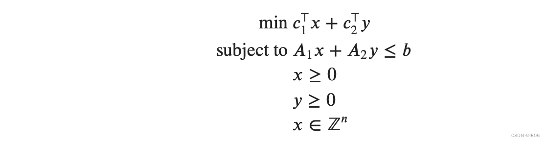
标准形如下,x是主问题变量,y是子问题变量:
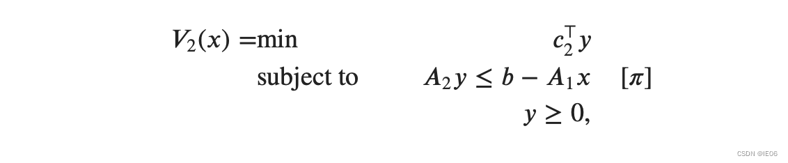
假设x已确定,将原问题做一个转换得到子问题:
每次迭代都是先用主问题求一个 x k x_k xk,然后代入子问题,得到对偶解 π k \pi_{k} πk,使用泰勒展开我们有

主问题变为:
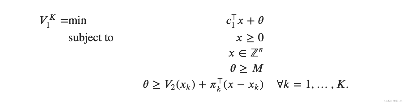
其中每一轮迭代添加一个约束
2. 求解步骤示例
这里还是举之前的例子:
max 2 w 1 + 3 w 2 + 2 w 3 + 5 w 4 + 2 w 5 + 6 w 6 \max 2 w_1+3w_2+2w_3+5w_4+2w_5+6w_6 max2w1+3w2+2w3+5w4+2w5+6w6
s.t. w 1 + w 2 + w 3 + w 4 ≤ − 2 w_1+w_2+w_3+w_4\le-2 w1+w2+w3+w4≤−2
w 2 + 2 w 4 ≤ − 1 w_2+2w_4\le-1 w2+2w4≤−1
w 1 − w 5 + 2 w 6 ≤ − 1 w_1-w_5+2w_6\le-1 w1−w5+2w6≤−1
2 w 2 + w 5 + w 6 ≤ 1 2w_2+w_5+w_6\le1 2w2+w5+w6≤1
w 1 . . . w 6 ≤ 0 w_1...w_6\le0 w1...w6≤0
分块如下:
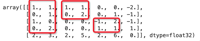
将 w 1 , w 2 w_1,w_2 w1,w2定义为主问题变量,4个约束通过对偶新增为4个新的隐变量,将目标函数用主问题变量和隐变量explicit表示出来为:
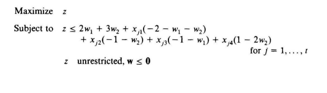
其中 x j 1 x_{j1} xj1~ x j 4 x_{j4} xj4是对偶问题的解。
第一轮迭代,只有主问题变量 w w w
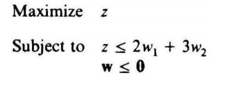
得到 w = ( 0 , 0 ) w=(0,0) w=(0,0), U B = 0 UB=0 UB=0,求解子问题(原问题子模块的对偶形式,不仅可以分块,而且是个线性规划问题):
min − 2 x 1 − x 2 − x 3 + x 4 \min -2x_1-x_2-x_3+x_4 min−2x1−x2−x3+x4
s.t.
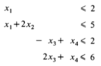
分块求解( x 1 , x 2 x_1,x_2 x1,x2)和( x 3 , x 4 x_3,x_4 x3,x4),可以得到 x = ( 2 , 1.5 , 3 , 0 ) x=(2,1.5,3,0) x=(2,1.5,3,0),最优值为 L B = − 8.5 LB=-8.5 LB=−8.5
第2轮迭代,使用新的 x x x添加一条约束,得到新的主问题:
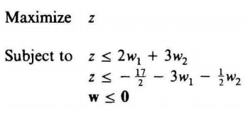
得到 w = ( − 1.7 , 0 ) w=(-1.7,0) w=(−1.7,0),最优值为 U B = − 3.4 UB=-3.4 UB=−3.4,带入目标函数求解子问题
min − 3.4 − 0.3 x 1 − x 2 − 2.7 x 3 + x 4 \min -3.4-0.3x_1-x_2-2.7x_3+x_4 min−3.4−0.3x1−x2−2.7x3+x4
s.t.
得到 x = ( 0 , 2.5 , 0 , 0 ) x=(0,2.5,0,0) x=(0,2.5,0,0),最优值为 L B = − 5.9 LB=-5.9 LB=−5.9
第3轮迭代,使用新的 x x x添加一条约束,得到新的主问题:
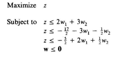
得到 w = ( − 1.2 , 0 ) w=(-1.2,0) w=(−1.2,0),最优值为 U B = − 4.9 UB=-4.9 UB=−4.9,求解子问题
min − 2.4 − 0.8 x 1 − x 2 + 0.2 x 3 + x 4 \min -2.4-0.8x_1-x_2+0.2x_3+x_4 min−2.4−0.8x1−x2+0.2x3+x4
s.t.
得到 x = ( 2 , 1.5 , 0 , 0 ) x=(2,1.5,0,0) x=(2,1.5,0,0),最优值为 L B = − 5.5 LB=-5.5 LB=−5.5
不断迭代下去即可,直到LB=UB
3. 参考代码
求解如下混合整数规划问题:
min x 1 + 4 x 2 + 2 x 3 + 3 x 4 \min x_1+4x_2+2x_3+3x_4 minx1+4x2+2x3+3x4
s.t. x 1 − 3 x 2 + x 3 − 2 x 4 ≤ − 2 x_1-3x_2+x_3-2x_4\le -2 x1−3x2+x3−2x4≤−2
− x 1 − 3 x 2 − x 3 − x 4 ≤ − 3 -x_1-3x_2-x_3-x_4\le -3 −x1−3x2−x3−x4≤−3
x 1 , x 2 ∈ Z x_1,x_2\in Z x1,x2∈Z
x 1 , . . . , x 4 ≥ 0 x_1,...,x_4\ge 0 x1,...,x4≥0
将 x 1 , x 2 x_1,x_2 x1,x2定义为主问题变量,数据如下:
c_1 = [1, 4]
c_2 = [2, 3]
dim_x = length(c_1)
dim_y = length(c_2)
b = [-2; -3]
A_1 = [1 -3; -1 -3]
A_2 = [1 -2; -1 -1]
M = -1000; #用于防治第一轮迭代找不到解
主问题和辅助函数如下:
model = Model(GLPK.Optimizer)
@variable(model, x[1:dim_x] >= 0, Int)
@variable(model, θ >= M)
@objective(model, Min, c_1' * x + θ)

MAXIMUM_ITERATIONS = 100
ABSOLUTE_OPTIMALITY_GAP = 1e-6
function print_iteration(k, args...)
    f(x) = Printf.@sprintf("%12.4e", x)
    println(lpad(k, 9), " ", join(f.(args), " "))
    return
end
3.1 使用迭代法
子问题如下
function solve_subproblem(x)
    model = Model(GLPK.Optimizer)
    @variable(model, y[1:dim_y] >= 0)
    con = @constraint(model, A_2 * y .<= b - A_1 * x)
    @objective(model, Min, c_2' * y)
    optimize!(model)
    return (obj = objective_value(model), y = value.(y), π = dual.(con))
end
迭代过程如下:
println("Iteration  Lower Bound  Upper Bound          Gap")
for k in 1:MAXIMUM_ITERATIONS
    optimize!(model)
    lower_bound = objective_value(model) #主问题是松弛问题,作为lb
    x_k = value.(x)
    ret = solve_subproblem(x_k)
    upper_bound = c_1' * x_k + ret.obj #子问题作为一个可行解,可以作为ub
    gap = (upper_bound - lower_bound) / upper_bound
    print_iteration(k, lower_bound, upper_bound, gap)
    if gap < ABSOLUTE_OPTIMALITY_GAP
        println("Terminating with the optimal solution")
        break
    end
    # 用子问题生成一个cut,添加到主问题上
    cut = @constraint(model, θ >= ret.obj + -ret.π' * A_1 * (x .- x_k))
    @info "Adding the cut $(cut)"
end

optimize!(model)
x_optimal = value.(x)
optimal_ret = solve_subproblem(x_optimal)
y_optimal = optimal_ret.y
3.2 使用lazy constraint
k = 0

"""
    my_callback(cb_data)

A callback that implements Benders decomposition. Note how similar it is to the
inner loop of the iterative method.
"""
function my_callback(cb_data)
    global k += 1
    x_k = callback_value.(cb_data, x)
    θ_k = callback_value(cb_data, θ)
    lower_bound = c_1' * x_k + θ_k
    ret = solve_subproblem(x_k)
    upper_bound = c_1' * x_k + c_2' * ret.y
    gap = (upper_bound - lower_bound) / upper_bound
    print_iteration(k, lower_bound, upper_bound, gap)
    if gap < ABSOLUTE_OPTIMALITY_GAP
        println("Terminating with the optimal solution")
        return
    end
    cut = @build_constraint(θ >= ret.obj + -ret.π' * A_1 * (x .- x_k))
    MOI.submit(model, MOI.LazyConstraint(cb_data), cut)
    return
end

MOI.set(lazy_model, MOI.LazyConstraintCallback(), my_callback)
x_optimal = value.(x)
optimal_ret = solve_subproblem(x_optimal)
y_optimal = optimal_ret.y
3.3 优化子问题模型
3.1节每次子问题都要重新建新模型求解,我们可以使用fix函数,直接利用原有的model进行求解:
function solve_subproblem(model, x)
    fix.(model[:x_copy], x)
    optimize!(model)
    @assert termination_status(model) == OPTIMAL
    return (
        obj = objective_value(model),
        y = value.(model[:y]),
        π = reduced_cost.(model[:x_copy]),
    )
end
这里的 π \pi π是x的剩余变量,添加约束的方式也有所变化:
println("Iteration  Lower Bound  Upper Bound          Gap")
for k in 1:MAXIMUM_ITERATIONS
    optimize!(model)
    lower_bound = objective_value(model)
    x_k = value.(x)
    ret = solve_subproblem(subproblem, x_k)
    upper_bound = c_1' * x_k + ret.obj
    gap = (upper_bound - lower_bound) / upper_bound
    print_iteration(k, lower_bound, upper_bound, gap)
    if gap < ABSOLUTE_OPTIMALITY_GAP
        println("Terminating with the optimal solution")
        break
    end
    cut = @constraint(model, θ >= ret.obj + ret.π' * (x .- x_k))
    @info "Adding the cut $(cut)"
end
和3.1节的区别在于:子问题多了x_copy部分,每次调用时使用fix函数,不需要重新构建模型。