全代码
纯手撸一个识别mnist手写数据集的2层DNN网络,所有库函数的低层NumPy代码都已给出,这串代码直接运行就能跑!不需要其他文件。
如果没装TensorFlow和matplotlib的童鞋可以在终端输入 pip install tensorflow 和 pip install matplotlib 进行安装。
import numpy as np
import matplotlib.pylab as plt
import tensorflow as tf #引入tensorflow只是为了导入mnist数据集
#下面一大段都是定义函数
def sigmoid(x):
return 1 / (1 + np.exp(-x))
def sigmoid_grad(x):
return (1.0 - sigmoid(x)) * sigmoid(x)
def relu(x):
return np.maximum(0, x)
def relu_grad(x):
#grad = np.zeros(x)
#grad[x>=0] = 1
x = np.where(x>=0,1,0)
return x
def softmax(x):
if x.ndim == 2:
x = x.T
x = x - np.max(x, axis=0)
y = np.exp(x) / np.sum(np.exp(x), axis=0)
return y.T
x = x - np.max(x) # 溢出对策
return np.exp(x) / np.sum(np.exp(x))
def mean_squared_error(y, t):
return 0.5 * np.sum((y - t) ** 2)
def cross_entropy_error(y, t):
if y.ndim == 1:
t = t.reshape(1, t.size)
y = y.reshape(1, y.size)
# 监督数据是one-hot-vector的情况下,转换为正确解标签的索引
if t.size == y.size:
t = t.argmax(axis=1)
batch_size = y.shape[0]
return -np.sum(np.log(y[np.arange(batch_size), t] + 1e-7)) / batch_size
def softmax_loss(X, t):
y = softmax(X)
return cross_entropy_error(y, t)
def numerical_gradient(f, x):
h = 1e-4 # 0.0001
grad = np.zeros_like(x)
it = np.nditer(x, flags=['multi_index'], op_flags=['readwrite'])
while not it.finished:
idx = it.multi_index
tmp_val = x[idx]
x[idx] = float(tmp_val) + h
fxh1 = f(x) # f(x+h)
x[idx] = tmp_val - h
fxh2 = f(x) # f(x-h)
grad[idx] = (fxh1 - fxh2) / (2 * h)
x[idx] = tmp_val # 还原值
it.iternext()
return grad
class TwoLayerNet:
def __init__(self, input_size, hidden_size, output_size, weight_init_std=0.01):
# 初始化权重
self.params = {
}
self.params['W1'] = weight_init_std * np.random.randn(input_size, hidden_size)
self.params['b1'] = np.zeros(hidden_size)
self.params['W2'] = weight_init_std * np.random.randn(hidden_size, output_size)
self.params['b2'] = np.zeros(output_size)
def predict(self, x):
W1, W2 = self.params['W1'], self.params['W2']
b1, b2 = self.params['b1'], self.params['b2']
a1 = np.dot(x, W1) + b1
#z1 = sigmoid(a1)
z1 = relu(a1)
a2 = np.dot(z1, W2) + b2
y = softmax(a2)
return y
# x:输入数据, t:监督数据
def loss(self, x, t):
y = self.predict(x)
return cross_entropy_error(y, t)
def accuracy(self, x, t):
y = self.predict(x)
y = np.argmax(y, axis=1)
t = np.argmax(t, axis=1)
accuracy = np.sum(y == t) / float(x.shape[0])
return accuracy
# x:输入数据, t:监督数据
def numerical_gradient(self, x, t):
loss_W = lambda W: self.loss(x, t)
grads = {
}
grads['W1'] = numerical_gradient(loss_W, self.params['W1'])
grads['b1'] = numerical_gradient(loss_W, self.params['b1'])
grads['W2'] = numerical_gradient(loss_W, self.params['W2'])
grads['b2'] = numerical_gradient(loss_W, self.params['b2'])
return grads
def gradient(self, x, t):
W1, W2 = self.params['W1'], self.params['W2']
b1, b2 = self.params['b1'], self.params['b2']
grads = {
}
batch_num = x.shape[0]
# forward
a1 = np.dot(x, W1) + b1
#z1 = sigmoid(a1)
z1 = relu(a1)
a2 = np.dot(z1, W2) + b2
y = softmax(a2)
# backward
dy = (y - t) / batch_num
grads['W2'] = np.dot(z1.T, dy)
grads['b2'] = np.sum(dy, axis=0)
da1 = np.dot(dy, W2.T)
#dz1 = sigmoid_grad(a1) * da1
dz1 = relu_grad(a1) * da1
grads['W1'] = np.dot(x.T, dz1)
grads['b1'] = np.sum(dz1, axis=0)
return grads
def _change_one_hot_label(X):
T = np.zeros((X.size, 10))
for idx, row in enumerate(T):
row[X[idx]] = 1
return T
#开搞
# 读入数据
mnist = tf.keras.datasets.mnist
(x_train, y_train), (x_test, y_test) = mnist.load_data()
x_train, x_test = x_train / 255.0, x_test / 255.0 #归一化
x_train = x_train.reshape(-1,784) # flatten, (60000,28,28)变(60000,784)
x_test = x_test.reshape(-1,784) # flatten, (10000,28,28)变(10000,784)
y_train = _change_one_hot_label(y_train) #标签变独热码,才能和前向传播softmax之后的结果维度匹配,才能相减算误差
y_test = _change_one_hot_label(y_test) #标签变独热码
#两层DNN(隐藏层50个神经元,784*50*10),激活函数是relu,可自己改成sigmoid,损失函数是交叉熵误差,输出层是softmax,优化函数是SGD
network = TwoLayerNet(input_size=784, hidden_size=50, output_size=10)
#超参数设置
iters_num = 10000
train_size = x_train.shape[0]
batch_size = 512
learning_rate = 0.05
train_loss_list = []
train_acc_list = []
test_acc_list = []
iter_per_epoch = max(train_size / batch_size, 1)
#训练
for i in range(iters_num):
batch_mask = np.random.choice(train_size, batch_size)
x_batch = x_train[batch_mask]
y_batch = y_train[batch_mask]
# 梯度
# grad = network.numerical_gradient(x_batch, t_batch)
grad = network.gradient(x_batch, y_batch)
# 更新
for key in ('W1', 'b1', 'W2', 'b2'):
network.params[key] -= learning_rate * grad[key]
loss = network.loss(x_batch, y_batch)
train_loss_list.append(loss)
#每一个epoch打印训练和测试的准确率
if i % iter_per_epoch == 0:
train_acc = network.accuracy(x_train, y_train)
test_acc = network.accuracy(x_test, y_test)
train_acc_list.append(train_acc)
test_acc_list.append(test_acc)
print(train_acc, test_acc)
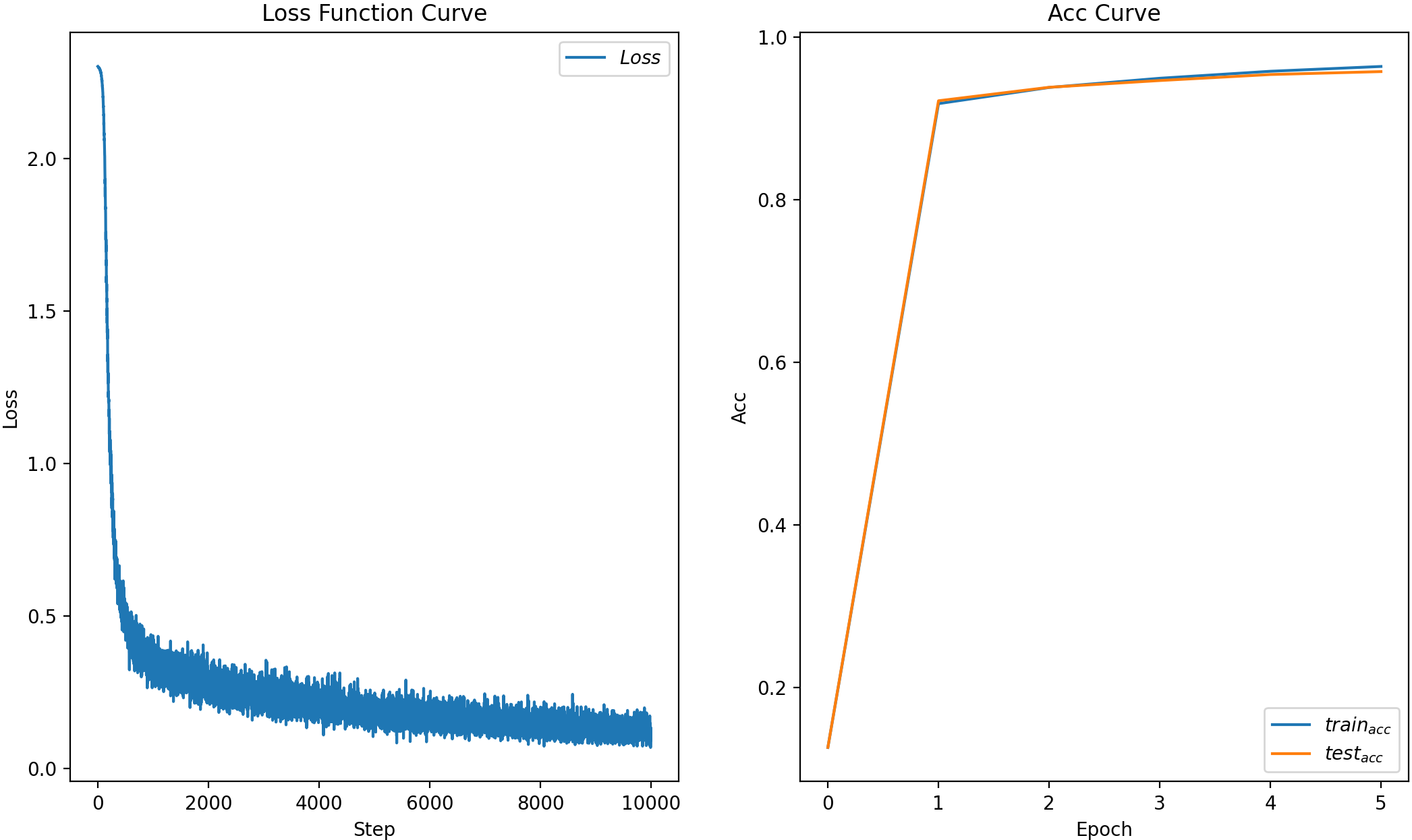
# 绘制 loss 曲线
plt.subplot(1,2,1)
plt.title('Loss Function Curve') # 图片标题
plt.xlabel('Step') # x轴变量名称
plt.ylabel('Loss') # y轴变量名称
plt.plot(train_loss_list, label="$Loss$") # 逐点画出loss值并连线,连线图标是Loss
plt.legend() # 画出曲线图标
# 绘制 Accuracy 曲线
plt.subplot(1,2,2)
plt.title('Acc Curve') # 图片标题
plt.xlabel('Epoch') # x轴变量名称
plt.ylabel('Acc') # y轴变量名称
plt.plot(train_acc_list, label="$train_{acc}$") # 逐点画出train_acc值并连线
plt.plot(test_acc_list, label="$test_{acc}$") # 逐点画出test_acc值并连线
plt.legend()
plt.show()
总结
简单的两层网络(W个数:784*50+50*10,b个数:50+10),就能实现95%的准确率,且没有过拟合。
batch_size调大一点loss就不会这么震荡,训练周期长一点acc会更大,学习率越大训练越快,但太大会跑飞,都可以调来玩玩。
上面的激活函数是选了relu,可自己改成sigmoid,代码里relu换成sigmoid就行,事实证明是relu好一点。
上面的优化器是SGD(随机梯度下降),还有Momentum、AdaGrad、Adam等等,一般用Adam会有更好效果。
所以可以总结神经网络学习全貌:
前提
神经网络存在合适的权重和偏置,调整权重和偏置以便拟合训练数据的
过程称为“学习”。神经网络的学习分成下面4个步骤。
步骤1(mini-batch)
从训练数据中随机选出一部分数据,这部分数据称为mini-batch。我们
的目标是减小mini-batch的损失函数的值。
步骤2(计算梯度)
扫描二维码关注公众号,回复:
14836021 查看本文章

为了减小mini-batch的损失函数的值,需要求出各个权重参数的梯度。
梯度表示损失函数的值减小最多的方向。
步骤3(更新参数)
将权重参数沿梯度方向进行微小更新。
步骤4(算误差、精度)
每次循环都算一下误差,若到一次epoch,算一下精度。
步骤5(重复)
重复步骤1、步骤2、步骤3、步骤4。
更多深度学习入门内容可以看看这篇哦《一文极速理解深度学习》。