【Python】可视化figure

1.Tensorboard静态显示

import torch
import torch.nn as nn
import matplotlib.pyplot as plt
import numpy as np
from torch.utils.tensorboard import SummaryWriter
import time
# ============================ step 1/5 生成数据 ============================
sample_nums = 100
mean_value = 1.7
bias = 1
n_data = torch.ones(sample_nums, 2)
# 使用正态分布随机生成样本，均值为张量，方差为标量
x0 = torch.normal(mean_value * n_data, 1) + bias      # 类别0 数据 shape=(100, 2)
# 生成对应标签
y0 = torch.zeros(sample_nums)                         # 类别0 标签 shape=(100, 1)
# 使用正态分布随机生成样本，均值为张量，方差为标量
x1 = torch.normal(-mean_value * n_data, 1) + bias     # 类别1 数据 shape=(100, 2)
# 生成对应标签
y1 = torch.ones(sample_nums)                          # 类别1 标签 shape=(100, 1)
train_x = torch.cat((x0, x1), 0)
train_y = torch.cat((y0, y1), 0)
i = 0
# ============================ step 2/5 选择模型 ============================
class LR(nn.Module):
    def __init__(self):
        super(LR, self).__init__()
        self.features = nn.Linear(2, 1)
        self.sigmoid = nn.Sigmoid()

    def forward(self, x):
        x = self.features(x)
        x = self.sigmoid(x)
        return x

lr_net = LR()   # 实例化逻辑回归模型

# ============================ step 3/5 选择损失函数 ============================
loss_fn = nn.BCELoss()

# ============================ step 4/5 选择优化器   ============================
lr = 0.01  # 学习率
optimizer = torch.optim.SGD(lr_net.parameters(), lr=lr, momentum=0.9)
writer = SummaryWriter("./runs/log")
# ============================ step 5/5 模型训练 ============================
for iteration in range(1000):

    # 前向传播
    y_pred = lr_net(train_x)
    # 计算 loss
    loss = loss_fn(y_pred.squeeze(), train_y)
    # 反向传播
    loss.backward()
    # 更新参数
    optimizer.step()
    # 清空梯度
    optimizer.zero_grad()
    # 绘图
    if iteration % 20 == 0:
        fig = plt.figure()
        mask = y_pred.ge(0.5).float().squeeze()  # 以0.5为阈值进行分类
        correct = (mask == train_y).sum()  # 计算正确预测的样本个数
        acc = correct.item() / train_y.size(0)  # 计算分类准确率

        plt.scatter(x0.data.numpy()[:, 0], x0.data.numpy()[:, 1], c='r', label='class 0')
        plt.scatter(x1.data.numpy()[:, 0], x1.data.numpy()[:, 1], c='b', label='class 1')

        w0, w1 = lr_net.features.weight[0]
        w0, w1 = float(w0.item()), float(w1.item())
        plot_b = float(lr_net.features.bias[0].item())
        plot_x = np.arange(-6, 6, 0.1)
        plot_y = (-w0 * plot_x - plot_b) / w1

        plt.xlim(-5, 7)
        plt.ylim(-7, 7)
        plt.plot(plot_x, plot_y)

        plt.text(-5, 5, 'Loss=%.4f' % loss.data.numpy(), fontdict={
    
    'size': 20, 'color': 'red'})
        plt.title("Iteration: {}\nw0:{:.2f} w1:{:.2f} b: {:.2f} accuracy:{:.2%}".format(iteration, w0, w1, plot_b, acc))
        plt.legend()
        # plt.savefig(str(iteration / 20)+".png")
        writer.add_figure('matplotlib', fig, i)
        i += 1
        time.sleep(0.1)
        # 如果准确率大于 99%，则停止训练
        if acc > 0.99:
            writer.close()
            break

(pytorch) C:\Users\rock\Desktop\2\STAR\src\runs>tensorboard --logdir=./log
TensorFlow installation not found - running with reduced feature set.
Serving TensorBoard on localhost; to expose to the network, use a proxy or pass --bind_all
TensorBoard 2.11.0 at http://localhost:6006/ (Press CTRL+C to quit)

2.Python动态显示

import torch
import torch.nn as nn
import matplotlib.pyplot as plt
import numpy as np
torch.manual_seed(10)
plt.ion() #开启interactive mode 成功的关键函数
# ============================ step 1/5 生成数据 ============================
sample_nums = 100
mean_value = 1.7
bias = 1
n_data = torch.ones(sample_nums, 2)
# 使用正态分布随机生成样本，均值为张量，方差为标量
x0 = torch.normal(mean_value * n_data, 1) + bias      # 类别0 数据 shape=(100, 2)
# 生成对应标签
y0 = torch.zeros(sample_nums)                         # 类别0 标签 shape=(100, 1)
# 使用正态分布随机生成样本，均值为张量，方差为标量
x1 = torch.normal(-mean_value * n_data, 1) + bias     # 类别1 数据 shape=(100, 2)
# 生成对应标签
y1 = torch.ones(sample_nums)                          # 类别1 标签 shape=(100, 1)
train_x = torch.cat((x0, x1), 0)
train_y = torch.cat((y0, y1), 0)

# ============================ step 2/5 选择模型 ============================
class LR(nn.Module):
    def __init__(self):
        super(LR, self).__init__()
        self.features = nn.Linear(2, 1)
        self.sigmoid = nn.Sigmoid()

    def forward(self, x):
        x = self.features(x)
        x = self.sigmoid(x)
        return x

lr_net = LR()   # 实例化逻辑回归模型

# ============================ step 3/5 选择损失函数 ============================
loss_fn = nn.BCELoss()

# ============================ step 4/5 选择优化器   ============================
lr = 0.01  # 学习率
optimizer = torch.optim.SGD(lr_net.parameters(), lr=lr, momentum=0.9)

# ============================ step 5/5 模型训练 ============================
for iteration in range(1000):

    # 前向传播
    y_pred = lr_net(train_x)
    # 计算 loss
    loss = loss_fn(y_pred.squeeze(), train_y)
    # 反向传播
    loss.backward()
    # 更新参数
    optimizer.step()
    # 清空梯度
    optimizer.zero_grad()
    # 绘图
    if iteration % 20 == 0:
        mask = y_pred.ge(0.5).float().squeeze()  # 以0.5为阈值进行分类
        correct = (mask == train_y).sum()  # 计算正确预测的样本个数
        acc = correct.item() / train_y.size(0)  # 计算分类准确率

        plt.scatter(x0.data.numpy()[:, 0], x0.data.numpy()[:, 1], c='r', label='class 0')
        plt.scatter(x1.data.numpy()[:, 0], x1.data.numpy()[:, 1], c='b', label='class 1')

        w0, w1 = lr_net.features.weight[0]
        w0, w1 = float(w0.item()), float(w1.item())
        plot_b = float(lr_net.features.bias[0].item())
        plot_x = np.arange(-6, 6, 0.1)
        plot_y = (-w0 * plot_x - plot_b) / w1

        plt.xlim(-5, 7)
        plt.ylim(-7, 7)
        plt.plot(plot_x, plot_y)

        plt.text(-5, 5, 'Loss=%.4f' % loss.data.numpy(), fontdict={
    
    'size': 20, 'color': 'red'})
        plt.title("Iteration: {}\nw0:{:.2f} w1:{:.2f} b: {:.2f} accuracy:{:.2%}".format(iteration, w0, w1, plot_b, acc))
        plt.legend()
        # plt.savefig(str(iteration / 20)+".png")
        plt.show()
        plt.pause(0.5)
        plt.clf()
        # 如果准确率大于 99%，则停止训练
        if acc > 0.99:
            break

tip:gif动图，如果不能播放刷新迅速回到此处可见，录制时没有设置自动回放。

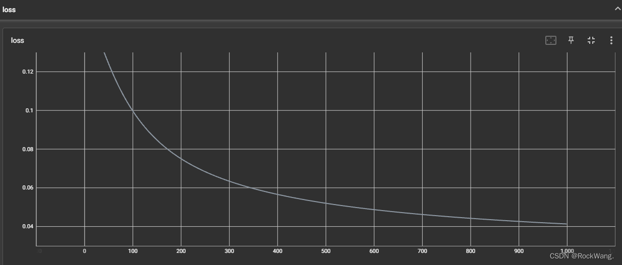
3.增加loss可视化

import torch
import torch.nn as nn
import matplotlib.pyplot as plt
import numpy as np
from torch.utils.tensorboard import SummaryWriter
import time
# ============================ step 1/5 生成数据 ============================
sample_nums = 100
mean_value = 1.7
bias = 1
n_data = torch.ones(sample_nums, 2)
# 使用正态分布随机生成样本，均值为张量，方差为标量
x0 = torch.normal(mean_value * n_data, 1) + bias      # 类别0 数据 shape=(100, 2)
# 生成对应标签
y0 = torch.zeros(sample_nums)                         # 类别0 标签 shape=(100, 1)
# 使用正态分布随机生成样本，均值为张量，方差为标量
x1 = torch.normal(-mean_value * n_data, 1) + bias     # 类别1 数据 shape=(100, 2)
# 生成对应标签
y1 = torch.ones(sample_nums)                          # 类别1 标签 shape=(100, 1)
train_x = torch.cat((x0, x1), 0)
train_y = torch.cat((y0, y1), 0)
i = 0
# ============================ step 2/5 选择模型 ============================
class LR(nn.Module):
    def __init__(self):
        super(LR, self).__init__()
        self.features = nn.Linear(2, 1)
        self.sigmoid = nn.Sigmoid()

    def forward(self, x):
        x = self.features(x)
        x = self.sigmoid(x)
        return x

lr_net = LR()   # 实例化逻辑回归模型

# ============================ step 3/5 选择损失函数 ============================
loss_fn = nn.BCELoss()

# ============================ step 4/5 选择优化器   ============================
lr = 0.01  # 学习率
optimizer = torch.optim.SGD(lr_net.parameters(), lr=lr, momentum=0.9)
writer = SummaryWriter("./runs/log")
# ============================ step 5/5 模型训练 ============================
for iteration in range(1000):

    # 前向传播
    y_pred = lr_net(train_x)
    # 计算 loss
    loss = loss_fn(y_pred.squeeze(), train_y)
    writer.add_scalar("loss", loss, iteration)
    # 反向传播
    loss.backward()
    # 更新参数
    optimizer.step()
    # 清空梯度
    optimizer.zero_grad()
    # 绘图
    if iteration % 20 == 0:
        fig = plt.figure()
        mask = y_pred.ge(0.5).float().squeeze()  # 以0.5为阈值进行分类
        correct = (mask == train_y).sum()  # 计算正确预测的样本个数
        acc = correct.item() / train_y.size(0)  # 计算分类准确率

        plt.scatter(x0.data.numpy()[:, 0], x0.data.numpy()[:, 1], c='r', label='class 0')
        plt.scatter(x1.data.numpy()[:, 0], x1.data.numpy()[:, 1], c='b', label='class 1')

        w0, w1 = lr_net.features.weight[0]
        w0, w1 = float(w0.item()), float(w1.item())
        plot_b = float(lr_net.features.bias[0].item())
        plot_x = np.arange(-6, 6, 0.1)
        plot_y = (-w0 * plot_x - plot_b) / w1

        plt.xlim(-5, 7)
        plt.ylim(-7, 7)
        plt.plot(plot_x, plot_y)

        plt.text(-5, 5, 'Loss=%.4f' % loss.data.numpy(), fontdict={
    
    'size': 20, 'color': 'red'})
        plt.title("Iteration: {}\nw0:{:.2f} w1:{:.2f} b: {:.2f} accuracy:{:.2%}".format(iteration, w0, w1, plot_b, acc))
        plt.legend()
        # plt.savefig(str(iteration / 20)+".png")
        writer.add_figure('matplotlib', fig, i)
        i += 1
        time.sleep(0.1)
        # 如果准确率大于 99%，则停止训练
        if acc > 0.99:
            writer.close()
            break