一、实验目的
通过鸢尾花萼片长度和宽度特征,采用感知器模型对鸢尾花数据集进行种类的分类识别。
二、算法步骤
1.数据准备
(1)从sklearn库里加载鸢尾花特性数据集;
iris = datasets.load_iris();
#[]内数字0、1、2、3分半表示花萼长、宽和花瓣长宽
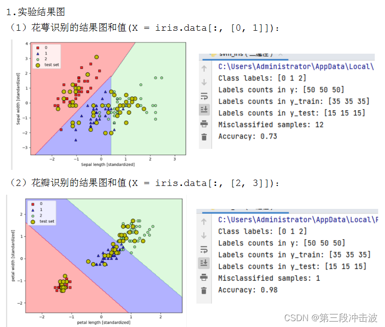
X = iris.data[:, [2, 3]]; y = iris.target;
# 打印输出的标签,0、1、2分别表示山鸢尾、变色鸢尾和维吉尼亚鸢尾。
print(‘Class labels:’, np.unique(y));
(2)用train_test_split函数将数据集随机分割成70%训练数据和30%测试数据, 并打印出三种花分别对应的所有数量、用于训练的数量和用于测试的数量,将训练数 据归一化,转换成一维数据保存在变量X_train_std和X_test_std中。
2.模型训练
对训练数据X_train_std和y_train采用svm进行数据拟合:
svm = SVC(kernel=‘linear’, C=1.0, random_state=1);
svm是线性拟合函数,其中,软间隔为1,随机状态为1.
3.数据绘图: 用plot_decision_regions函数将150条数据和45条测试数据显示在一张图上,分别用’s’(红),’^’(蓝),‘o’(绿)和’O’(黄)表示0类、1类、2类花和测试的数据标注。
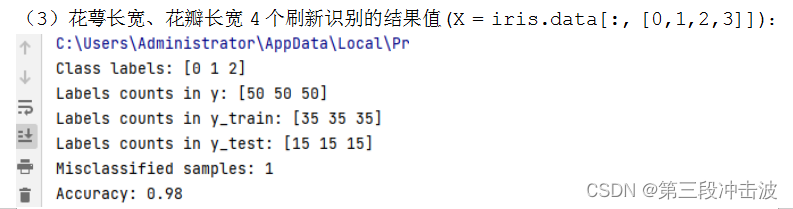
4.模型评估: 打印出测试集中错误分类的样本的个数Misclassified samples,与测试集整体识别的准确率Accuracy。
print(‘Misclassified samples: %d’ % (y_test != y_pred).sum())
print(‘Accuracy: %.2f’ % svm.score(X_test_std, y_test))
三、直接上代码
from sklearn import __version__ as sklearn_version
from distutils.version import LooseVersion
from sklearn import datasets
import numpy as np
from sklearn.model_selection import train_test_split
from sklearn.preprocessing import StandardScaler
from sklearn.linear_model import Perceptron
from sklearn.metrics import accuracy_score
from matplotlib.colors import ListedColormap
import matplotlib.pyplot as plt
from sklearn.linear_model import LogisticRegression
from sklearn.svm import SVC
from sklearn.neighbors import KNeighborsClassifier

iris = datasets.load_iris()
X = iris.data[:, [2, 3]]
y = iris.target

print('Class labels:', np.unique(y))


# Splitting data into 70% training and 30% test data:


X_train, X_test, y_train, y_test = train_test_split(
    X, y, test_size=0.3, random_state=1, stratify=y)


print('Labels counts in y:', np.bincount(y))
print('Labels counts in y_train:', np.bincount(y_train))
print('Labels counts in y_test:', np.bincount(y_test))

sc = StandardScaler()
sc.fit(X_train)
X_train_std = sc.transform(X_train)
X_test_std = sc.transform(X_test)

def plot_decision_regions(X, y, classifier, test_idx=None, resolution=0.02):

    # setup marker generator and color map
    markers = ('s', '^', 'o', 'x', 'v')
    colors = ('red', 'blue', 'lightgreen', 'gray', 'cyan')
    cmap = ListedColormap(colors[:len(np.unique(y))])

    # plot the decision surface
    x1_min, x1_max = X[:, 0].min() - 1, X[:, 0].max() + 1
    x2_min, x2_max = X[:, 1].min() - 1, X[:, 1].max() + 1
    xx1, xx2 = np.meshgrid(np.arange(x1_min, x1_max, resolution),
                           np.arange(x2_min, x2_max, resolution))
    Z = classifier.predict(np.array([xx1.ravel(), xx2.ravel()]).T)
    Z = Z.reshape(xx1.shape)
    plt.contourf(xx1, xx2, Z, alpha=0.3, cmap=cmap)
    plt.xlim(xx1.min(), xx1.max())
    plt.ylim(xx2.min(), xx2.max())

    for idx, cl in enumerate(np.unique(y)):
        plt.scatter(x=X[y == cl, 0],
                    y=X[y == cl, 1],
                    alpha=0.8,
                    c=colors[idx],
                    marker=markers[idx],
                    label=cl,
                    edgecolor='black')

    # highlight test samples
    # if test_idx:
    #     # plot all samples
    #     X_test, y_test = X[test_idx, :], y[test_idx]
    #
    #     plt.scatter(X_test[:, 0],
    #                 X_test[:, 1],
    #                 c='y',
    #                 edgecolor='black',
    #                 alpha=1.0,
    #                 linewidth=1,
    #                 marker='o',
    #                 s=100,
    #                 label='test set')

# Training a svm model using the standardized training data:


X_combined_std = np.vstack((X_train_std, X_test_std))
y_combined = np.hstack((y_train, y_test))


svm = SVC(kernel='linear', C=1.0, random_state=1)
svm.fit(X_train_std, y_train)

plot_decision_regions(X_combined_std,
                      y_combined,
                      classifier=svm,
                      test_idx=range(105, 150))
plt.xlabel('petal length [standardized]')
plt.ylabel('petal width [standardized]')
plt.legend(loc='upper left')
plt.tight_layout()
#plt.savefig('images/03_11.png', dpi=300)
plt.show()

y_pred = svm.predict(X_test_std)
print('Misclassified samples: %d' % (y_test != y_pred).sum())
print('Accuracy: %.2f' % svm.score(X_test_std, y_test))
四、实验结果