这里写目录标题
1.给出一个线性回归模型并求出因子贡献度
##-----------------------------------------------------------------------------
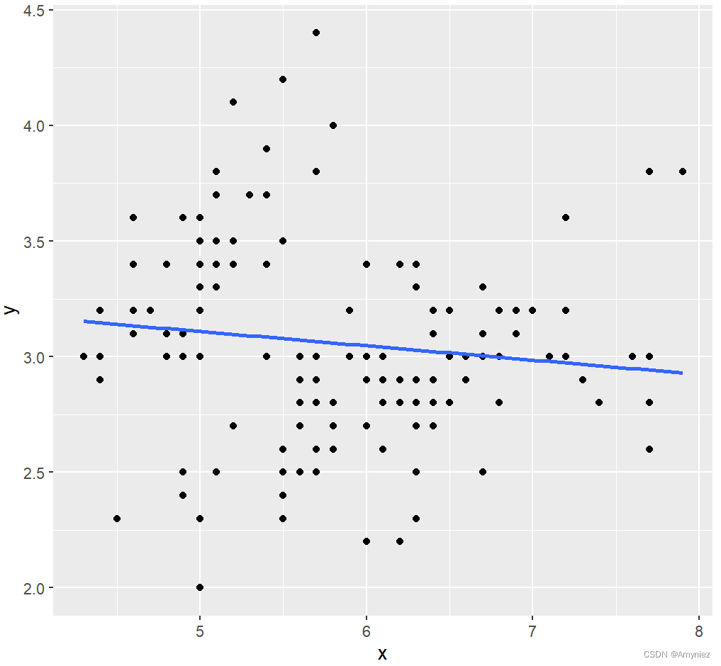
# 线性回归模型
lm_df <- data.frame(x = iris$Sepal.Length,y = iris$Sepal.Width)
lm_model <- lm(data = lm_df,y ~ x)
broom::tidy(lm_model)
ggplot(data = lm_df,aes(x,y))+
geom_point()+
geom_smooth(method = lm, se = FALSE)
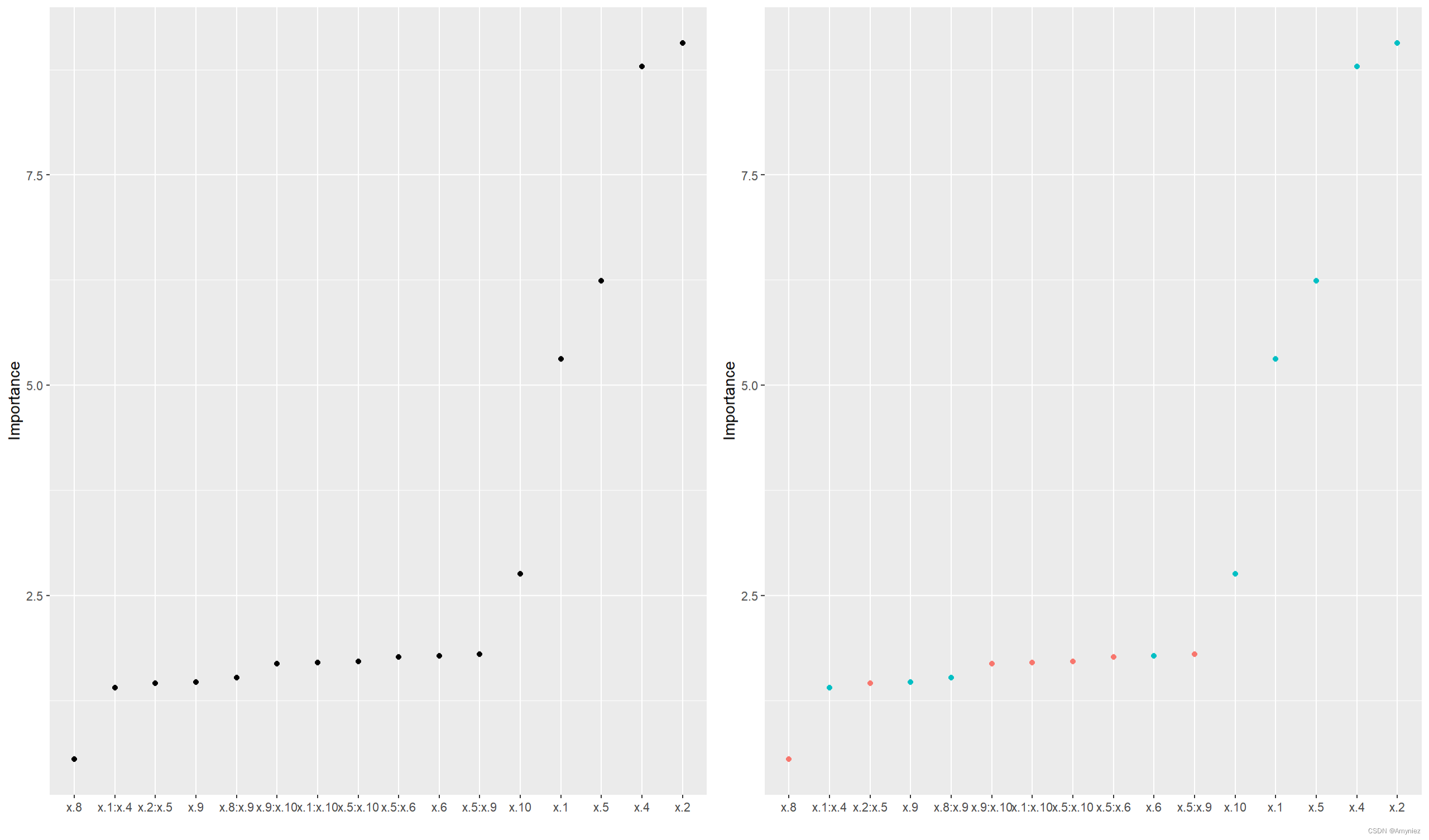
# 变量重要性
install.packages("vip")
install.packages('mlbench')
library(vip)
set.seed(100)
trn <- as.data.frame(mlbench::mlbench.friedman1(500))
linmod <- lm(y ~ .^2, data = trn)
backward <- step(linmod, direction = "backward", trace = 0)
# 计算贡献度
vi(backward)
# 可视化
p1 <- vip(backward, num_features = length(coef(backward)),
geom = "point", horizontal = FALSE)
p2 <- vip(backward, num_features = length(coef(backward)),
geom = "point", horizontal = FALSE,
mapping = aes_string(color = "Sign"))
grid.arrange(p1, p2, nrow = 1)
结果展示:

图像绘制:
重要性结果展示:
2.biomod2
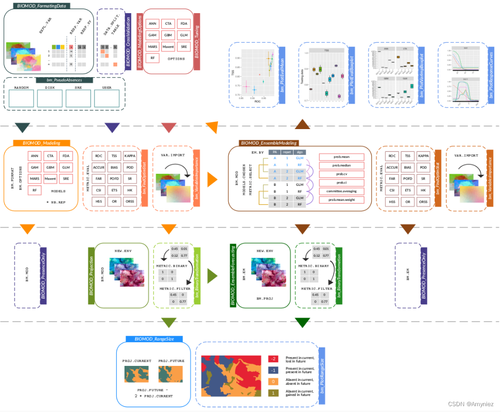
首先需要安装biomod2包:install.packages(“biomod2”)
最终生成的文件为individual_projections,该文件夹中包括.img、.xml两种数据格式,其中包括很多算法如,GLM,RF,SRE,ANN,CTA,FDA,CTA等多种模型 ,这类似于一个集成算法,集合多个模型,求取模型的平均值,以得出一个更好的模型。
##-----------------------------------------------------------------------------
# 加载成都市的适量边界图,后面会用到
library(mapchina)
cd_sf <- mapchina::china %>%
  dplyr::filter(Name_Perfecture == "成都市") %>%
  group_by(Name_Province) %>%
  summarise(geometry = sf::st_union(geometry)) %>%
  ungroup()
colnames(cd_sf) # see all variable names
plot(cd_sf)

#install.packages("biomod2")
library(biomod2)

?biomod2::BIOMOD_FormatingData()
#
2.1 pseudo-absences:伪不存在点(PA)
生成PA点的四种方法:random、disk、sre、user.table
2.1.1 random
随机选择PA点
##--------------------------------------------------------------------------------
# 1.the random method : PA are randomly selected over the studied area (excluding presence points)
library(sf)
p1_random <- sf::st_sample(cd_sf,300)
ggplot()+
  geom_sf(data = cd_sf)+
  geom_sf(data = p1_random)
结果展示:
2.2.2 disk
# 2.the disk method : PA are randomly selected within circles around presence
#   points defined by a minimum and a maximum distance values (defined in meters).
## Format Data with pseudo-absences : disk method
# myBiomodData.d <- BIOMOD_FormatingData(resp.var = myResp.PA,
#                                        expl.var = myExpl,
#                                        resp.xy = myRespXY,
#                                        resp.name = myRespName,
#                                        PA.nb.rep = 4,
#                                        PA.nb.absences = 500,
#                                        PA.strategy = 'disk',
#                                        PA.dist.min = 5,
#                                        PA.dist.max = 35) # 生成环形缓冲区
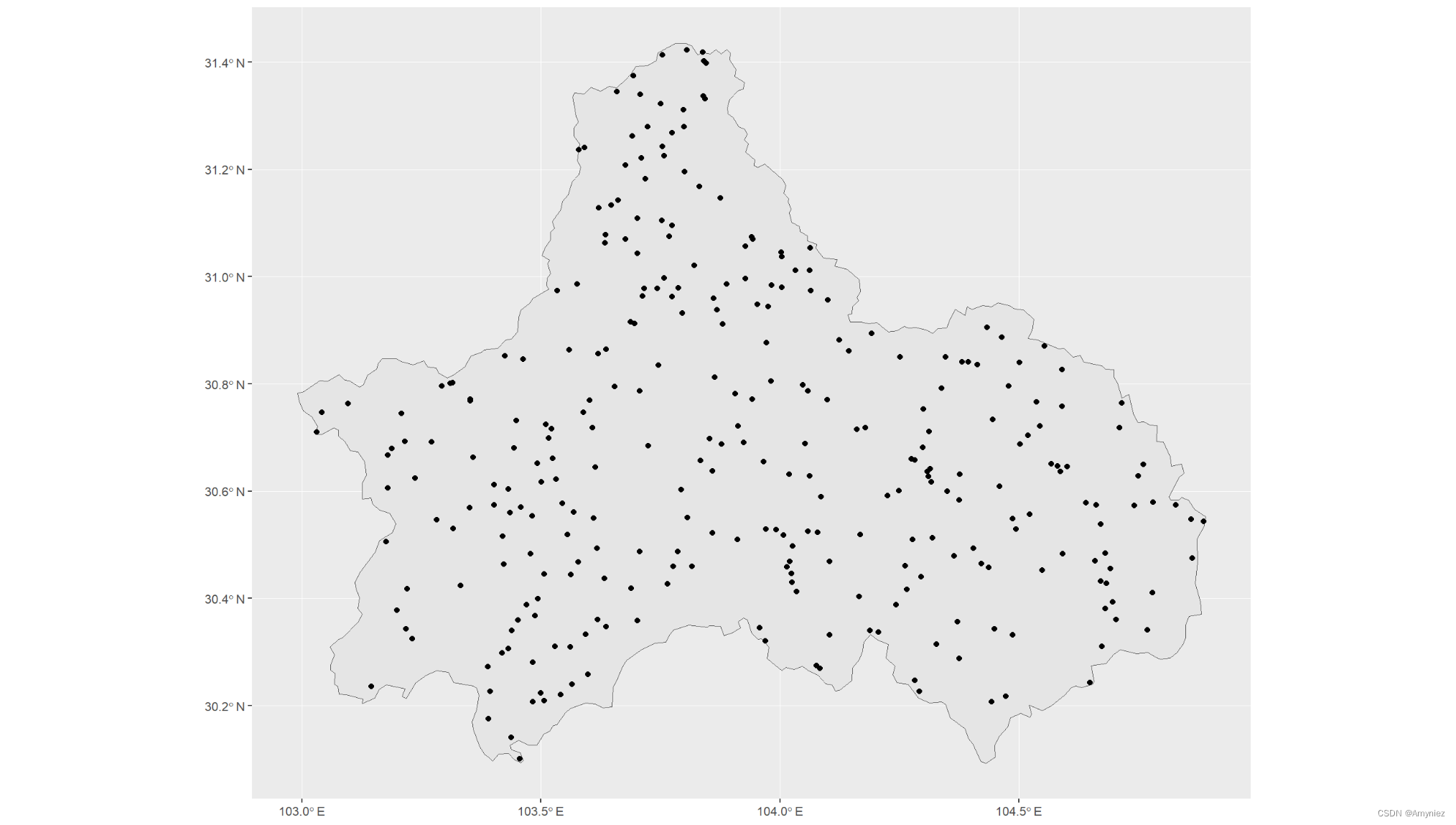
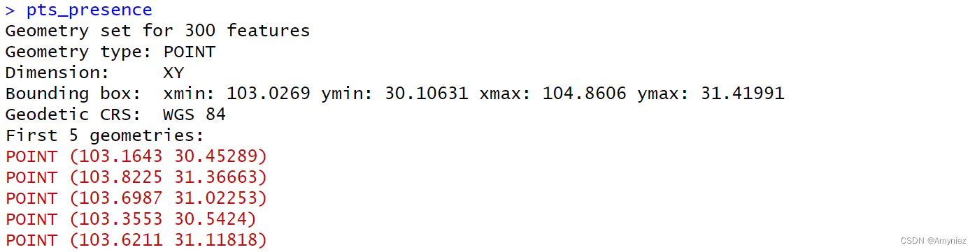
pts_presence <- sf::st_sample(cd_sf,300)
pts_presence
#使用生成的第一个点画圆
st_buffer(pts_presence[[1]], dist = 1) %>% plot()
plot(pts_presence[[1]],add = TRUE)
结果展示:

2.2.3 user.defined method
##-------------------------------------------------------------------------------------
#用户自定义
## Format Data with pseudo-absences : user.defined method
# myPAtable <- data.frame(PA1 = ifelse(myResp == 1, TRUE, FALSE),
#                         PA2 = ifelse(myResp == 1, TRUE, FALSE))
# for (i in 1:ncol(myPAtable)) myPAtable[sample(which(myPAtable[, i] == FALSE), 500), i] = TRUE
# myBiomodData.u <- BIOMOD_FormatingData(resp.var = myResp.PA,
#                                        expl.var = myExpl,
#                                        resp.xy = myRespXY,
#                                        resp.name = myRespName,
#                                        PA.strategy = 'user.defined',
#                                        PA.user.table = myPAtable)
pts_absence <- pts_presence %>%
  st_as_sf() %>%
  mutate(id = 1:n()) %>%
  group_by(id) %>%
  nest(data = -id) %>%
  mutate(circle = purrr::map(.x = data,.f = function(x) {


    st_buffer(x = x,dist = 1)
  })) %>%
  mutate(point = purrr::map(.x = circle,.f = function(x) {


    st_sample(x,1)
  })) %>%
  dplyr::select(point) %>%
  unnest() %>%
  ungroup() %>%
  dplyr::select(-id)
pts_absence

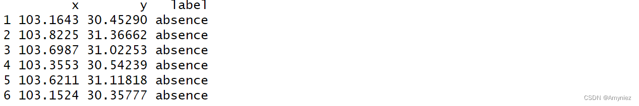
格式转换:
# 将生成的点转换为数据框格式
#install.packages('sfheaders')
library(sfheaders)
pts_absence %>%
  st_as_sf() %>%
  sfheaders::sf_to_df() %>%
  dplyr::select(x,y) %>%
  mutate(label = "absence") %>%
  head()
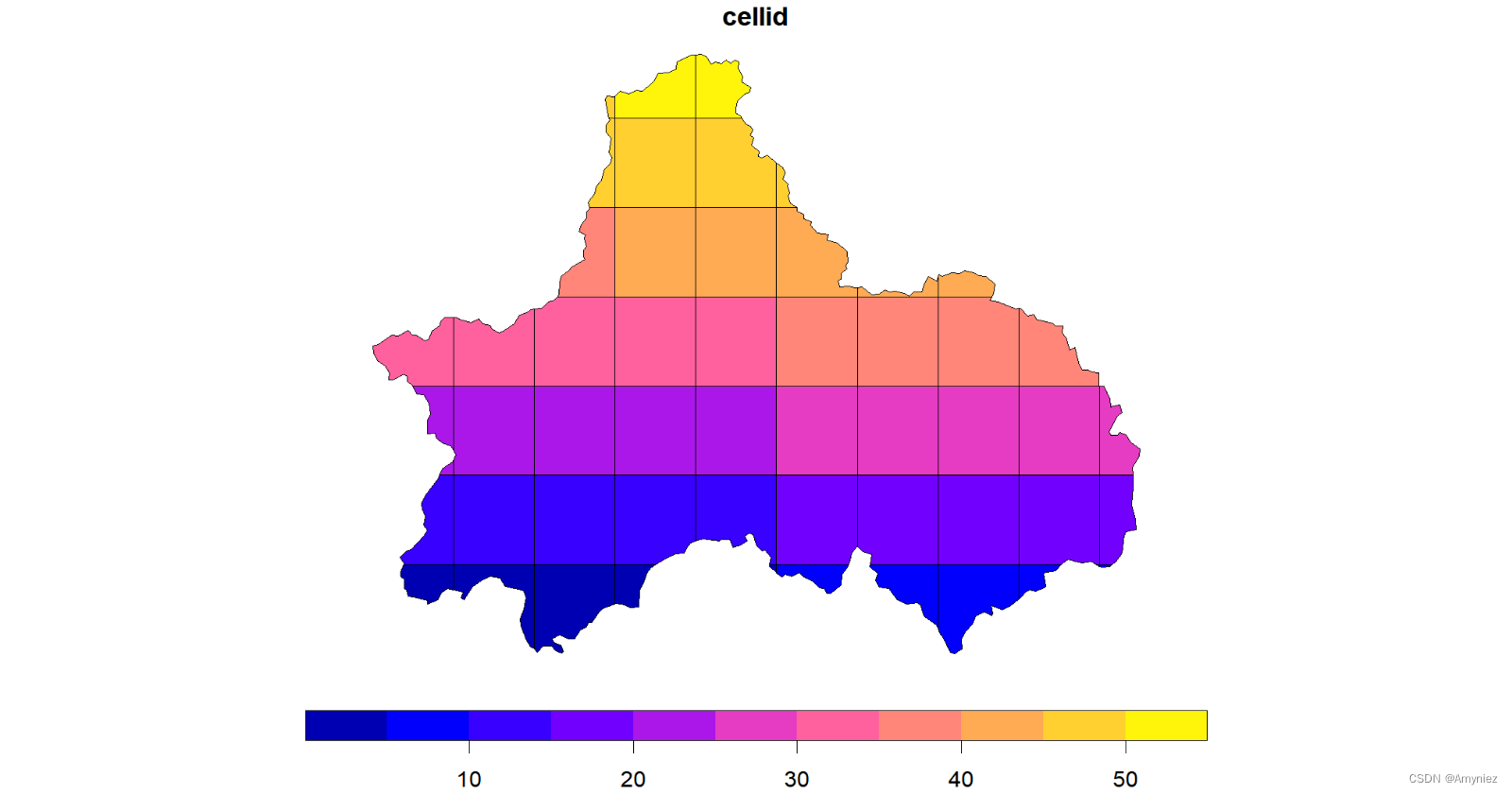
3.使用网格划分区域
##----------------------------------------------------------------------------------
# 网格划分,形成栅格图像
cd_grid <- cd_sf %>%
  st_make_grid(cellsize = 0.2) %>%
  st_intersection(cd_sf) %>%
  st_cast("MULTIPOLYGON") %>%
  st_sf() %>%
  mutate(cellid = row_number())
plot(cd_grid)
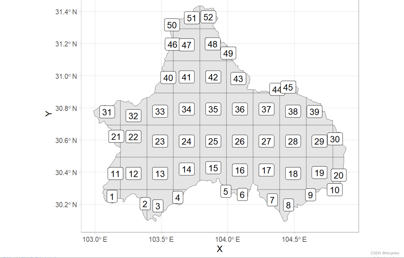
为每个网格添加标签:
#devtools::install_github("yutannihilation/ggsflabel")
ggplot(data = cd_grid)+
  geom_sf()+
  ggsflabel::geom_sf_label(aes(label = cellid))+
  theme_light()
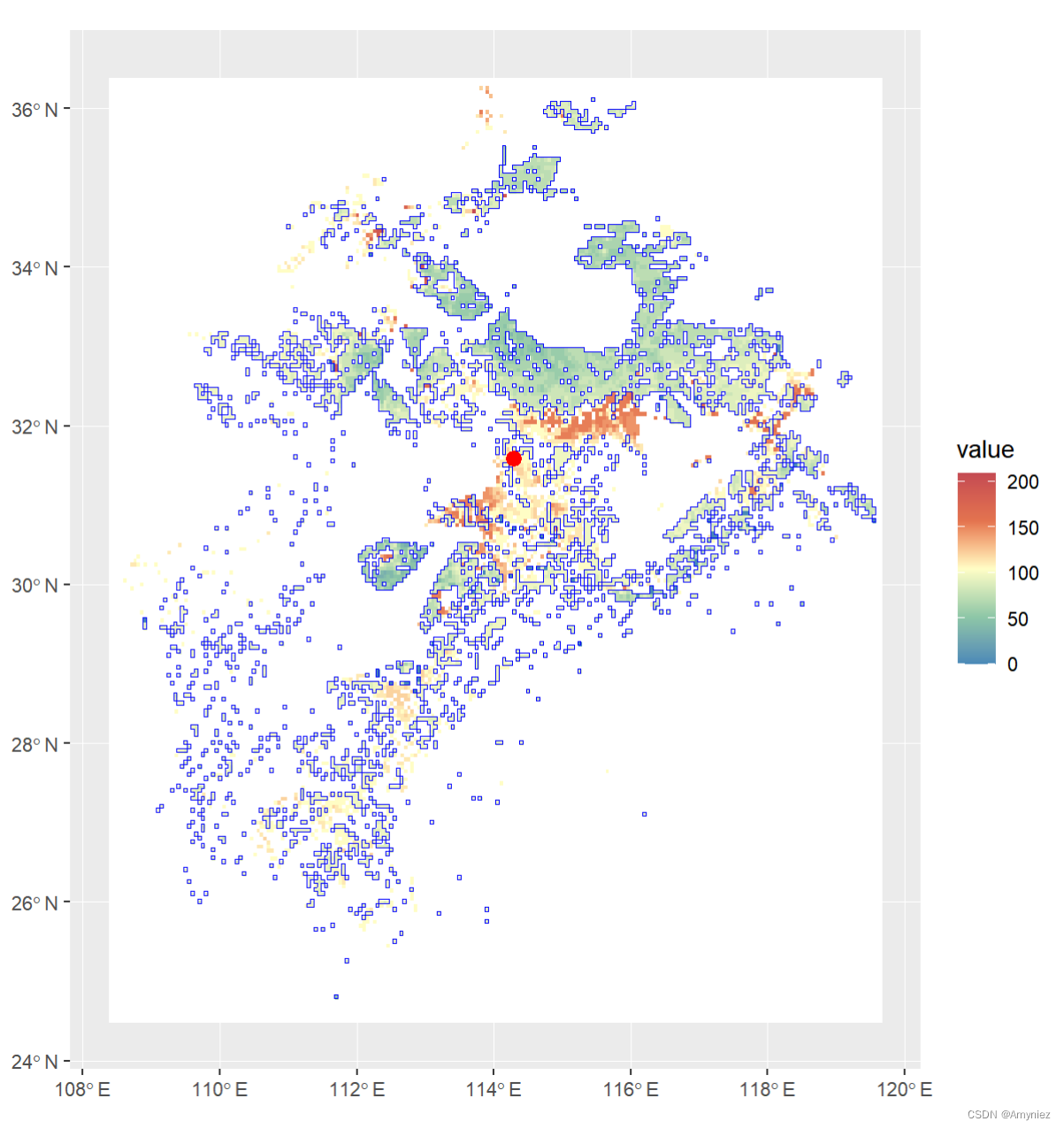
3.1 计算质心
# 计算质心
library(terra)
library(tidyterra)
library(ggplot2)
bj_dem <- raster("D:/Datasets/w001001.adf")
plot(bj_dem)
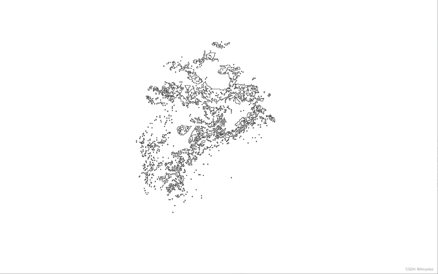
(sp_sf <- bj_dem %>%
calc(x = .,fun = function(x) ifelse(x < 100,x,NA)) %>% # 按属性筛选
rasterToPolygons() %>%
st_as_sf() %>%
summarise(geometry = st_union(geometry)) %>%
st_make_valid())
plot(sp_sf)
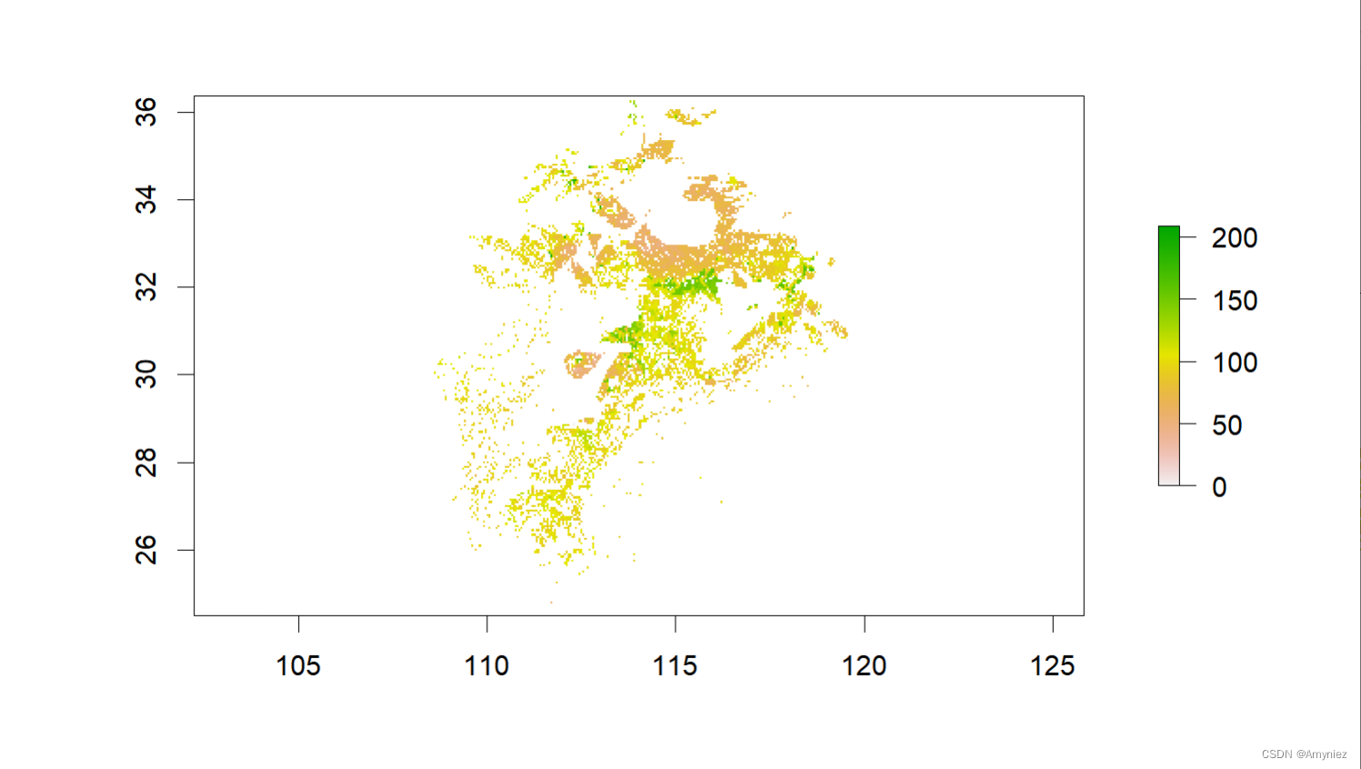
centroid <- st_centroid(sp_sf)

ggplot()+
  geom_spatraster(data = rast(bj_dem)) +
  scale_fill_whitebox_c(
    palette = "muted",
    na.value = "white"
  )+
  geom_sf(data = sp_sf,alpha = 0,color = "blue")+
  geom_sf(data = centroid,size = 3,color = "red")
4. 完整案例
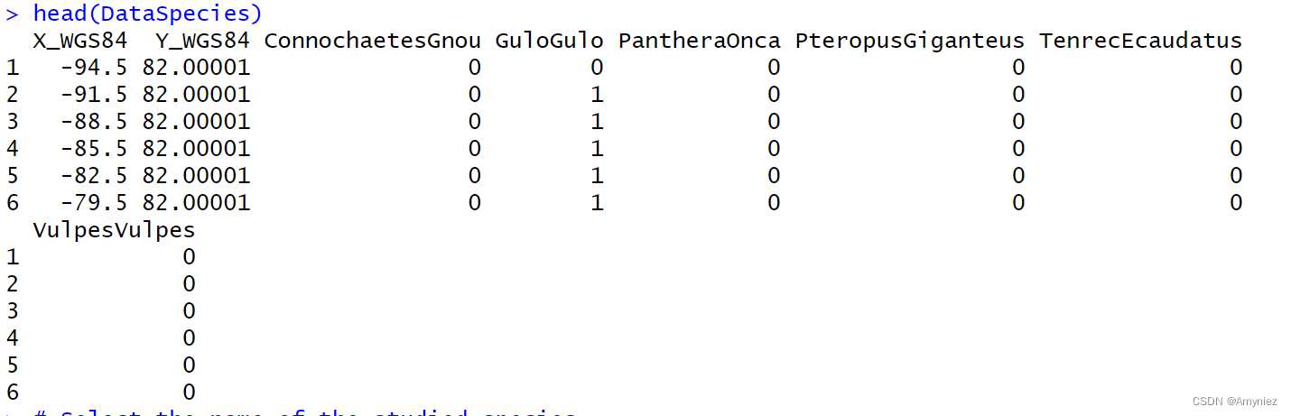
# Load species occurrences (6 species available)
data(DataSpecies)
head(DataSpecies)
# Select the name of the studied species
myRespName <- 'GuloGulo'
# Get corresponding presence/absence data
myResp <- as.numeric(DataSpecies[, myRespName])
# Get corresponding XY coordinates
myRespXY <- DataSpecies[, c('X_WGS84', 'Y_WGS84')]
# Load environmental variables extracted from BIOCLIM (bio_3, bio_4, bio_7, bio_11 & bio_12)
data(bioclim_current)
myExpl <- terra::rast(bioclim_current)
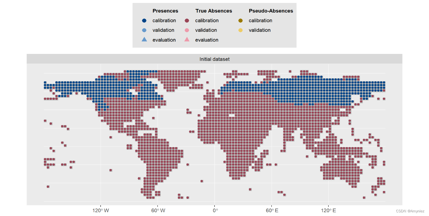
## --------------------------------------------------------------------------------
# Format Data with true absences
myBiomodData <- BIOMOD_FormatingData(resp.var = myResp,
expl.var = myExpl,
resp.xy = myRespXY,
resp.name = myRespName)
myBiomodData
summary(myBiomodData)
plot(myBiomodData)
物种分布数据: