hello, 今天聊一聊ISP当中的一个重要模块CCM;
Color Correction Matrix (CCM)
The Color Correction Matrix block corrects the image color variations coming from many different causes that can include spectral characteristics of the optics (lens, filters), lighting source variations, characteristics of the color filters of the sensor and many others. The CCM block contains 3x3 programmable coefficient matrix multipliers with offset compensation that can be used in color correction operations such as adjusting white balance, color cast, brightness, or contrast in an image.
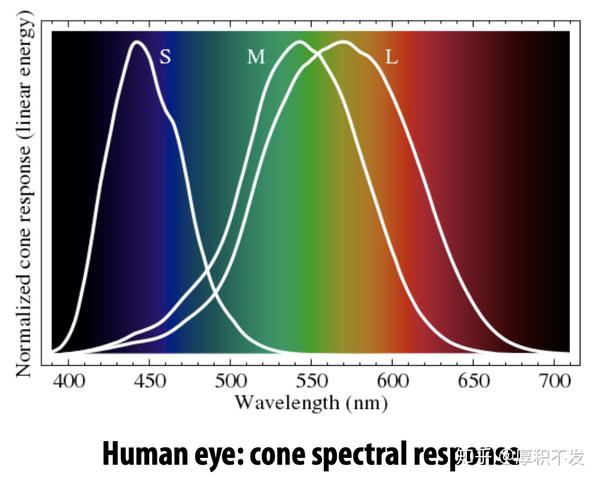
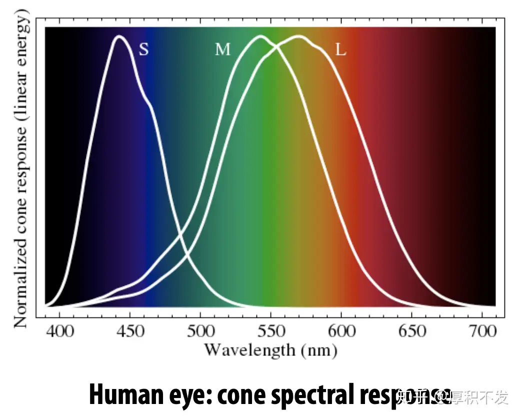
为什么ISP模块中要有这个模块呢,上面列的一堆原因,最重要的因素是我们肉眼的对光谱的RGB响应曲线和sensor的响应曲线是不同的;
CCM一般是3x3矩阵形式,也有3x4形式的,3x4形式主要是给rgb各自加一个offset
[RoutGoutBout]=[CC00CC01CC02CC10CC11CC12CC20CC21CC22]∗[RinGintBin]CC_{00} + CC_{01} + CC_{02} = 1\\ CC_{10} + CC_{11} + CC_{12} = 1\\ CC_{20} + CC_{21} + CC_{22} = 1
保证灰点也就是r=g=b的点,经过CCM以后仍然r=g=b;
标定CCM方法:
- 用camera拍一张某个色温下的24色卡raw文件:
注意shading影响,拍这个色卡占整个sensor中间一小部分就可以


- raw文件预处理
主要包括减blc,根据第4行的patch,获取awb gain值,乘上去;这样就拿到了这个色温下24个patch的rgb值;
- 理想rgb值
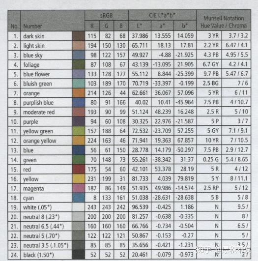

这是色卡厂家提供的24个patch的标准rgb空间下的理论值;
拿到这个值以后,需要进行反gamma处理,因为厂家提供的是srgb的值,是带了2.2gamma的,ISP的CCM模块一般是在gamma前面,因此要对理论值进行反gamma处理;
现在准备工作完成了,接下来是算法;
标定算法
已知100个raw rgb值,已知对应的理论rgb值;求一个3x3线性变换矩阵;这个矩阵要使得映射后的rgb值尽可能的接近理论值;
借鉴深度学习的梯度下降方法,可以快速得到CCM;并且可以自定义100个patch的重要程度,使得某些patch的误差非常小。
抱歉手头没有24色卡的raw,没有真实数据;只能用随机数据来模拟了;
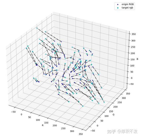
首先我们随机生成18个随机rgb值,定义一个矩阵,画出它的映射:
import matplotlib.pyplot as plt
import torch
ccm = torch.tensor([[1655, -442, -189], [-248, 1466, -194], [-48, -770, 1842]], dtype=torch.float32)
rgb_data = torch.randint(0, 255, (3, 100))
rgb_data = rgb_data.float()
rgb_target = ccm.mm(rgb_data)/1024.0
fig1 = plt.figure(1)
ax1 = fig1.add_subplot(111, projection=‘3d’)
x2 = rgb_data[0]
y2 = rgb_data[1]
z2 = rgb_data[2]
ax1.scatter(x2, y2, z2, marker=‘*’, c=‘b’, label=‘origin RGB’)
ax1.set_xlim(-80, 360)
ax1.set_ylim(-80, 360)
ax1.set_zlim(-80, 360)
ax1.set_xlabel(‘R’)
ax1.set_ylabel(‘G’)
ax1.set_zlabel(‘B’)
x3 = rgb_target[0]
y3 = rgb_target[1]
z3 = rgb_target[2]
ax1.scatter(x3, y3, z3, marker=‘o’, c=‘c’, label=‘target rgb’)
for i in range(len(x3)):
ax1.plot([x2[i], x3[i]], [y2[i], y3[i]], [z2[i], z3[i]], ‘k-.’)
ax1.legend()
plt.show()
映射关系如下:

现在给原始rgb加一些noise,根据上面得到的CCM后的rgb值,来推算CCM,看是否和预定义的CCM接近:
error_manual = torch.randn((3, 100))  16

rgb_target_error = rgb_target + error_manual
定义损失和梯度函数,测量rgb值得差异,采用L2距离;
L_{i} = \sum_{n=1}^{18}(CCM*RGB_{origin}- RGB_{standard})^2
完整代码如下:
from mpl_toolkits.mplot3d import Axes3D

import matplotlib.pyplot as plt

import torch
ccm = torch.tensor([[1655, -442, -189], [-248, 1466, -194], [-48, -770, 1842]], dtype=torch.float32)
rgb_data = torch.randint(0, 255, (3, 100))
rgb_data = rgb_data.float()
error_manual = torch.randn((3, 100)) * 16
rgb_target = ccm.mm(rgb_data)/1024.0
rgb_target_error = rgb_target + error_manual
ccm_calc1 = torch.tensor([0.0], dtype=torch.float32, requires_grad=True)
ccm_calc2 = torch.tensor([0.0], dtype=torch.float32, requires_grad=True)
ccm_calc3 = torch.tensor([0.0], dtype=torch.float32, requires_grad=True)
ccm_calc5 = torch.tensor([0.0], dtype=torch.float32, requires_grad=True)
ccm_calc6 = torch.tensor([0.0], dtype=torch.float32, requires_grad=True)
ccm_calc7 = torch.tensor([0.0], dtype=torch.float32, requires_grad=True)
def squared_loss(rgb_tmp, rgb_ideal):
return torch.sum((rgb_tmp-rgb_ideal)**2)
def sgd(params, lr, batch_size):
for param in params:
param.data -= lr * param.grad/batch_size;
def net(ccm_calc1, ccm_calc2, ccm_calc3, ccm_calc5, ccm_calc6, ccm_calc7, rgb_data):
rgb_tmp = torch.zeros_like(rgb_data)
rgb_tmp[0, :] = ((1024.0 - ccm_calc1 - ccm_calc2) rgb_data[0, :] + ccm_calc1 rgb_data[1, :] + ccm_calc2 rgb_data[2, :]) / 1024.0
rgb_tmp[1, :] = (ccm_calc3 rgb_data[0, :] + (1024.0 - ccm_calc3 - ccm_calc5) rgb_data[1, :] + ccm_calc5 rgb_data[2, :]) / 1024.0
rgb_tmp[2, :] = (ccm_calc6 rgb_data[0, :] + ccm_calc7 rgb_data[1, :] + (1024.0 - ccm_calc6 - ccm_calc7) * rgb_data[2, :]) / 1024.0
return rgb_tmp
lr = 3
num_epochs = 100
for epoch in range(num_epochs):
l = squared_loss(net(ccm_calc1, ccm_calc2, ccm_calc3, ccm_calc5, ccm_calc6, ccm_calc7, rgb_data), rgb_target_error)
l.backward()
sgd([ccm_calc1, ccm_calc2, ccm_calc3, ccm_calc5, ccm_calc6, ccm_calc7], lr, 100)
ccm_calc1.grad.data.zero_()
ccm_calc2.grad.data.zero_()
ccm_calc3.grad.data.zero_()
ccm_calc5.grad.data.zero_()
ccm_calc6.grad.data.zero_()
ccm_calc7.grad.data.zero_()
print(‘epoch %d, loss %f’%(epoch, l))
res = torch.tensor([[1024.0 - ccm_calc1 - ccm_calc2, ccm_calc1, ccm_calc2],
[ccm_calc3, 1024.0-ccm_calc3-ccm_calc5, ccm_calc5],
[ccm_calc6, ccm_calc7, 1024.0-ccm_calc6-ccm_calc7]], dtype=torch.float32)
print(res);
rgb_apply_ccm = res.mm(rgb_data)/1024.0
fig1 = plt.figure(1)
ax1 = fig1.add_subplot(111, projection=‘3d’)
fig2 = plt.figure(2)
ax2 = fig2.add_subplot(111, projection=‘3d’)
x2 = rgb_data[0]
y2 = rgb_data[1]
z2 = rgb_data[2]
ax1.scatter(x2, y2, z2, marker=‘*’, c=‘b’, label=‘origin RGB’)
ax1.set_xlim(-80, 360)
ax1.set_ylim(-80, 360)
ax1.set_zlim(-80, 360)
ax1.set_xlabel(‘R’)
ax1.set_ylabel(‘G’)
ax1.set_zlabel(‘B’)
x3 = rgb_target[0]
y3 = rgb_target[1]
z3 = rgb_target[2]
ax1.scatter(x3, y3, z3, marker=‘o’, c=‘c’, label=‘target rgb’)
for i in range(len(x3)):
ax1.plot([x2[i], x3[i]], [y2[i], y3[i]], [z2[i], z3[i]], ‘k-.’)
ax1.legend()
ax2.set_xlim(-80, 360)
ax2.set_ylim(-80, 360)
ax2.set_zlim(-80, 360)
ax2.set_xlabel(‘R’)
ax2.set_ylabel(‘G’)
ax2.set_zlabel(‘B’)
ax2.scatter(x3, y3, z3, marker=‘o’, c=‘c’, label=‘target rgb’)
x4 = rgb_apply_ccm[0]
y4 = rgb_apply_ccm[1]
z4 = rgb_apply_ccm[2]
ax2.scatter(x4, y4, z4, marker=‘^’, c=‘b’, label=‘apply ccm rgb’)
ax2.legend()
plt.show()
运行结果对比:
可视化看一下映射后的点与理论点的距离:
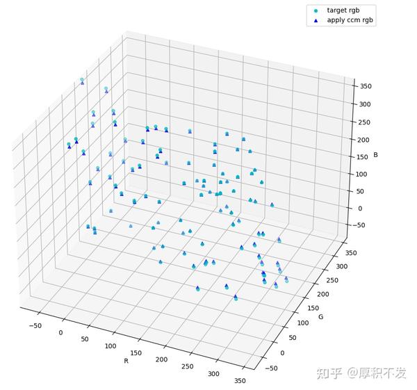

很接近了!!!
如果觉得对你有帮助,请点个赞,点个关注,谢谢!