文章目录
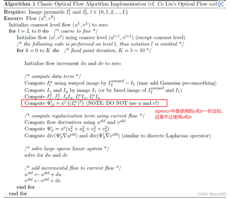
1.Fast Optical Flow using Dense Inverse Search
该篇论文是求dense flow,效果和速度都很好,虽然有源码(opencv上也有),但是网上的介绍不是很多,不是很容易理解。
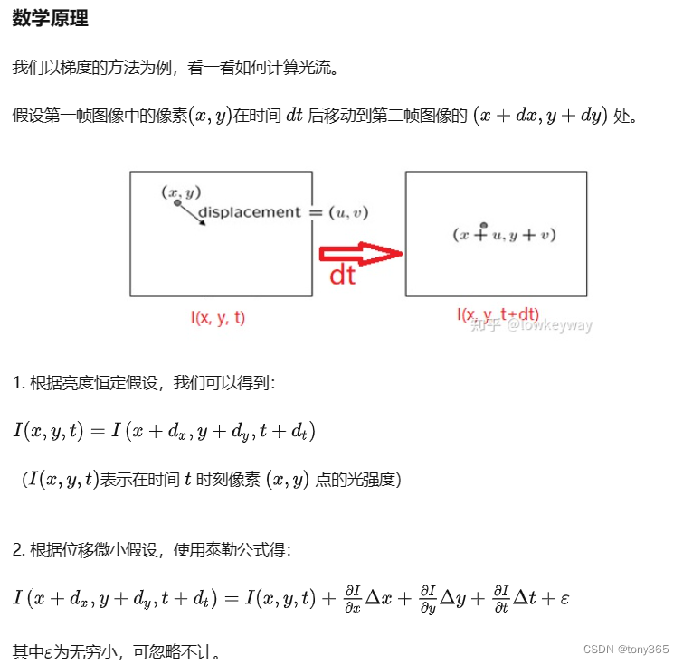
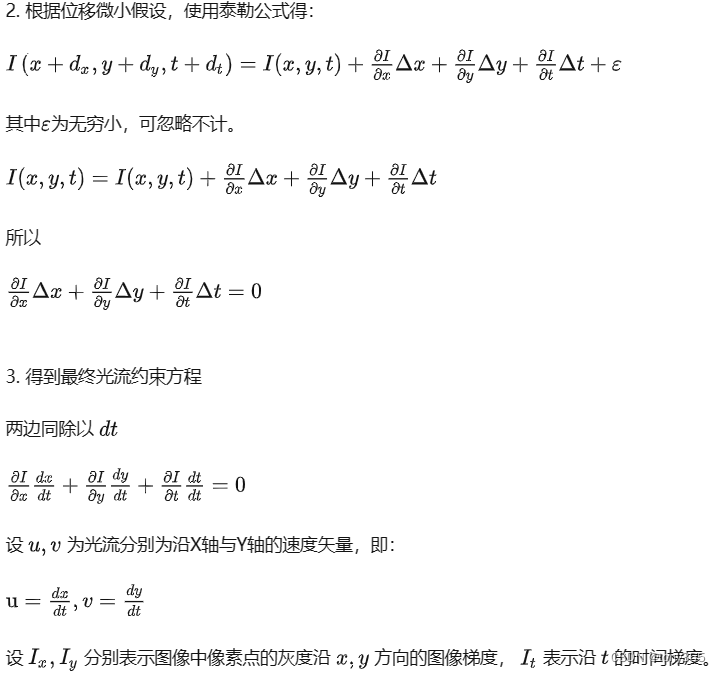
要想理解该论文,首先要理解光流法
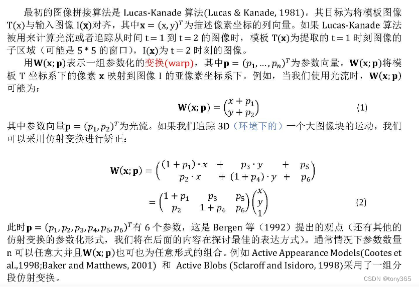
1.1 W的含义:
对于光流来说 W 表示光流:x方向上的光流u,y方向上的光流v
同时W也可以表示更复杂的坐标变换方法,比如affine仿射变换
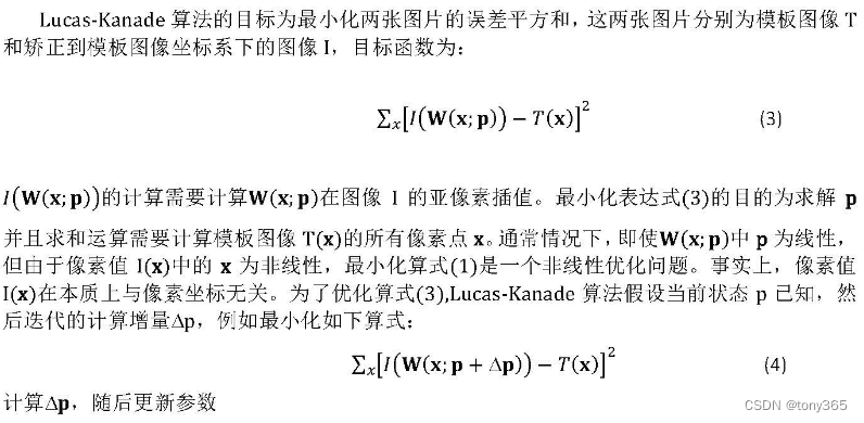
1.2 LK光流模型
对图像2进行warp 与 图像1相减。
利用迭代的方法更新和优化

1.3 LK光流模型求解(不含迭代)
1.4 LK光流模型迭代求解
在4.2中提到迭代求解的光流模型
I 0 ( x , y ) = I 1 ( x + u , y + v ) I0(x,y) = I1(x+u, y+v) I0(x,y)=I1(x+u,y+v)变为 I 0 ( x , y ) = I 1 ( x + u + d u , y + v + d v ) I0(x,y) = I1(x+u+du, y+v+dv) I0(x,y)=I1(x+u+du,y+v+dv)
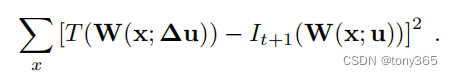
优化目标为:
m i n ∣ ∣ I 0 ( x , y ) − I 1 ( x + u + d u , y + v + d v ) ∣ ∣ 2 min ||I0(x,y)-I1(x+u+du, y+v+dv)||^2 min∣∣I0(x,y)−I1(x+u+du,y+v+dv)∣∣2
令 I 0 ( x , y ) − I 1 ( x + u + d u , y + v + d v ) = 0 I0(x,y)-I1(x+u+du, y+v+dv) = 0 I0(x,y)−I1(x+u+du,y+v+dv)=0
I 1 ( x + u + d u , y + v + d v ) = I 1 ( x + u , y + v ) + I 1 ( x + u , y + v ) x d u + I 1 ( x + u , y + v ) y d v I1(x+u+du, y+v+dv) = I1(x+u, y+v) + I1(x+u, y+v)_x du + I1(x+u, y+v)_y dv I1(x+u+du,y+v+dv)=I1(x+u,y+v)+I1(x+u,y+v)xdu+I1(x+u,y+v)ydv
令 I 1 w a r p = I 1 ( x + u , y + v ) I1warp = I1(x+u, y+v) I1warp=I1(x+u,y+v)
已知上一次迭代u,v光流,或者初始设为0,可以求出 I 1 w a r p I1warp I1warp
则 I 1 ( x + u + d u , y + v + d v ) = I 1 w a r p + I 1 w a r p x d u + I 1 w a r p y d v I1(x+u+du, y+v+dv) = I1warp + I1warp_x du + I1warp_y dv I1(x+u+du,y+v+dv)=I1warp+I1warpxdu+I1warpydv
然后:
I 0 ( x , y ) − I 1 ( x + u + d u , y + v + d v ) = 0 I 0 ( x , y ) − I 1 w a r p + I 1 w a r p x d u + I 1 w a r p y d v = 0 I 1 w a r p x d u + I 1 w a r p y d v = I 0 ( x , y ) − I 1 w a r p I 1 w a r p x d u + I 1 w a r p y d v = I z I0(x,y)-I1(x+u+du, y+v+dv)=0 \\ I0(x,y) - I1warp + I1warp_x du + I1warp_y dv =0\\ I1warp_x du + I1warp_y dv = I0(x,y) - I1warp\\ I1warp_x du + I1warp_y dv = Iz I0(x,y)−I1(x+u+du,y+v+dv)=0I0(x,y)−I1warp+I1warpxdu+I1warpydv=0I1warpxdu+I1warpydv=I0(x,y)−I1warpI1warpxdu+I1warpydv=Iz
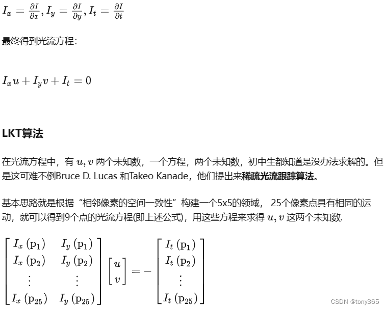
假设对于一个patchsize = 8邻域内的点, du, dv是相同的
则可以建立线性方程组,然后同4.3可通过最小二乘法求得 d u , d v du, dv du,dv
I 1 w a r p x ( p 1 ) d u + I 1 w a r p y ( p 1 ) d v = I z ( p 1 ) I 1 w a r p x ( p 2 ) d u + I 1 w a r p y ( p 2 ) d v = I z ( p 2 ) I 1 w a r p x ( p 2 ) d u + I 1 w a r p y ( p 2 ) d v = I z ( p 2 ) . . . I 1 w a r p x ( p 64 ) d u + I 1 w a r p y ( p 64 ) d v = I z ( p 64 ) I1warp_x(p1) du + I1warp_y(p1) dv = Iz(p1)\\ I1warp_x(p2) du + I1warp_y(p2) dv = Iz(p2)\\ I1warp_x(p2) du + I1warp_y(p2) dv = Iz(p2)\\ ...\\ I1warp_x(p64) du + I1warp_y(p64) dv = Iz(p64) I1warpx(p1)du+I1warpy(p1)dv=Iz(p1)I1warpx(p2)du+I1warpy(p2)dv=Iz(p2)I1warpx(p2)du+I1warpy(p2)dv=Iz(p2)...I1warpx(p64)du+I1warpy(p64)dv=Iz(p64)
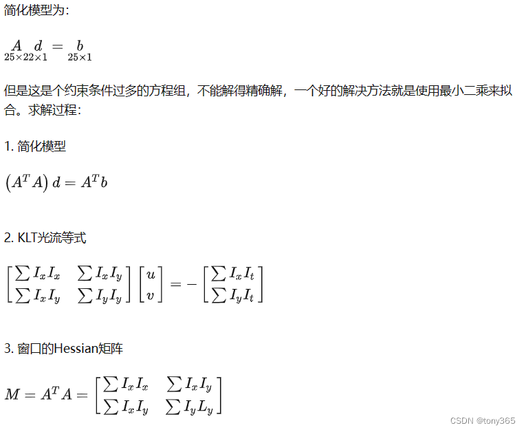
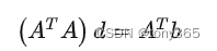
可建立 A d = b Ad=b Ad=b
其中
A = [ I 1 w a r p x ( p 1 ) I 1 w a r p y ( p 1 ) I 1 w a r p x ( p 2 ) I 1 w a r p y ( p 2 ) . . . I 1 w a r p x ( p n ) I 1 w a r p y ( p n ) ] A=\left[ \begin{array}{ccc} I1warp_x(p1) \qquad I1warp_y(p1)\\ I1warp_x(p2) \qquad I1warp_y(p2)\\ ...\\ I1warp_x(pn) \qquad I1warp_y(pn)\\ \end{array} \right ] A=
I1warpx(p1)I1warpy(p1)I1warpx(p2)I1warpy(p2)...I1warpx(pn)I1warpy(pn)
d = [ d u d v ] d=\left[ \begin{array}{ccc} du\\ dv \end{array} \right ] d=[dudv]
b = [ I z ( p 1 ) I z ( p 2 ) . . . I z ( p n ) ] b=\left[ \begin{array}{ccc} Iz(p1)\\ Iz(p2)\\ ...\\ Iz(pn) \end{array} \right ] b= Iz(p1)Iz(p2)...Iz(pn)
最小二乘法
H = [ ∑ I 1 w a r p x × I 1 w a r p x ∑ I 1 w a r p x × I 1 w a r p y ∑ I 1 w a r p x × I 1 w a r p y ∑ I 1 w a r p y × I 1 w a r p y ] H=\left[ \begin{array}{ccc} \sum I1warp_x\times I1warp_x & \sum I1warp_x\times I1warp_y\\ \sum I1warp_x\times I1warp_y & \sum I1warp_y\times I1warp_y\\ \end{array} \right ] H=[∑I1warpx×I1warpx∑I1warpx×I1warpy∑I1warpx×I1warpy∑I1warpy×I1warpy]
B = A T b = [ ∑ I 1 w a r p x I z ∑ I 1 w a r p y I z ] B=A^Tb = \left[ \begin{array}{ccc} \sum I1warp_x Iz\\ \sum I1warp_y Iz \end{array} \right ] B=ATb=[∑I1warpxIz∑I1warpyIz]
d = H − 1 × B d = H^{-1} \times B d=H−1×B
最后更新
u = u + d u v = v + d v u = u+du\\ v=v+dv u=u+duv=v+dv
以及 I1warp也要更新
1.5 dis_flow方法中的 LK光流模型
在4.4中,每次求出du,dv后首先更新u,v,然后更新I1warp
还要根据I1warp更新方程组的参数 I 1 w a r p x , I 1 w a r p y I1warp_x ,I1warp_y I1warpx,I1warpy
等于说是每次迭代都要重新算梯度。
而dis_flow方法采用下面的模型:
即每次求出 du, dv之后,并不是作用在 I1warp中,而是作用在 I0 中,当然光流也是相反的方向
I 0 ( x + d u , y + d v ) − I 1 ( x + u , y + v ) = 0 I 0 ( x , y ) + I 0 x d u + I 0 y d v − I 1 ( x + u , y + v ) = 0 I0(x+du, y+dv)-I1(x+u,y+v)=0\\ I0(x,y)+I0_xdu+I0_ydv-I1(x+u,y+v)=0 I0(x+du,y+dv)−I1(x+u,y+v)=0I0(x,y)+I0xdu+I0ydv−I1(x+u,y+v)=0
可以得到
I 0 x d u + I 0 y d v = I 1 ( x + u , y + v ) − I 0 ( x , y ) I0_xdu + I0_ydv = I1(x+u,y+v)-I0(x,y) I0xdu+I0ydv=I1(x+u,y+v)−I0(x,y)
同理可以求得 H 和 b,进而求出 du, dv
H = [ ∑ I 0 x × I 0 x ∑ I 0 x × I 0 y ∑ I 0 x × I 0 y ∑ I 0 y × I 0 y ] H=\left[ \begin{array}{ccc} \sum I0_x\times I0_x & \sum I0_x\times I0_y\\ \sum I0_x\times I0_y & \sum I0_y\times I0_y\\ \end{array} \right ] H=[∑I0x×I0x∑I0x×I0y∑I0x×I0y∑I0y×I0y]
B = A T b = [ ∑ I 0 x I z ∑ I 0 y I z ] B=A^Tb = \left[ \begin{array}{ccc} \sum I0_x Iz\\ \sum I0_y Iz \end{array} \right ] B=ATb=[∑I0xIz∑I0yIz]
d = H − 1 × B d = H^{-1} \times B d=H−1×B
更新 u = u − d u , v = v − d v u=u-du, v=v-dv u=u−du,v=v−dv 记住这里是相减,因为du,dv是对I0而言的,作用在I1上符号变号
更新 I 1 ( x + u , y + v ) I1(x+u,y+v) I1(x+u,y+v)
然后再次循环求解,H矩阵是由I0的梯度求的,而不是I1warp的梯度求得,因此不需要每次迭代更新,只需更新一次,大大减少计算量。
加入以上是针对一个小patch优化求解 u,v, 可以设置步长便利整个图像,得到每个patch的u,v如果patch有重叠,则加权平均。
最终得到每个像素点光流u,v
1.6 disflow代码分析
看代码的确实是这样:
1)computeSSD 函数计算 两个patch的ssd,
2)computeSSDMeanNorm 返回的 是 两个patch减去各自均值后的 SSD, 避免亮度差异对ssd的影响
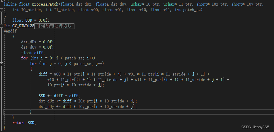
3)processPatch 函数 计算两个patch的ssd, 且 计算 dst_dUx, dst_dUy
对应的是
B = A T b = [ ∑ I 0 x I z ∑ I 0 y I z ] B=A^Tb = \left[ \begin{array}{ccc} \sum I0_x Iz\\ \sum I0_y Iz \end{array} \right ] B=ATb=[∑I0xIz∑I0yIz]
diff对应的是 I 1 w a r p − I 0 I1warp - I0 I1warp−I0
4)processPatchMeanNorm 函数是先均值归一化,在计算。
5)precomputeStructureTensor函数计算好每个patch的 地图平方和
对应的是H中的元素
H = [ ∑ I 0 x × I 0 x ∑ I 0 x × I 0 y ∑ I 0 x × I 0 y ∑ I 0 y × I 0 y ] H=\left[ \begin{array}{ccc} \sum I0_x\times I0_x & \sum I0_x\times I0_y\\ \sum I0_x\times I0_y & \sum I0_y\times I0_y\\ \end{array} \right ] H=[∑I0x×I0x∑I0x×I0y∑I0x×I0y∑I0y×I0y]
    Mat_<float> I0xx_buf; //!< sum of squares of x gradient values
    Mat_<float> I0yy_buf; //!< sum of squares of y gradient values
    Mat_<float> I0xy_buf; //!< sum of x and y gradient products

    /* Extra buffers that are useful if patch mean-normalization is used: */
    Mat_<float> I0x_buf; //!< sum of x gradient values
    Mat_<float> I0y_buf; //!< sum of y gradient values
6) void DISOpticalFlowImpl::PatchInverseSearch_ParBody::operator()(const Range &range) const
函数中有每个patch的迭代过程:
计算 H − 1 H^{-1} H−1
/* Precomputed structure tensor */
float *xx_ptr = dis->I0xx_buf.ptr<float>();
float *yy_ptr = dis->I0yy_buf.ptr<float>();
float *xy_ptr = dis->I0xy_buf.ptr<float>();
/* And extra buffers for mean-normalization: */
float *x_ptr = dis->I0x_buf.ptr<float>();
float *y_ptr = dis->I0y_buf.ptr<float>();

 /* Use the best candidate as a starting point for the gradient descent: */
float cur_Ux = Sx_ptr[is * dis->ws + js];
float cur_Uy = Sy_ptr[is * dis->ws + js];

/* Computing the inverse of the structure tensor: */
float detH = xx_ptr[is * dis->ws + js] * yy_ptr[is * dis->ws + js] -
                xy_ptr[is * dis->ws + js] * xy_ptr[is * dis->ws + js];
if (abs(detH) < EPS)
    detH = EPS;
float invH11 = yy_ptr[is * dis->ws + js] / detH;
float invH12 = -xy_ptr[is * dis->ws + js] / detH;
float invH22 = xx_ptr[is * dis->ws + js] / detH;
计算 dUx, dUy, 就是
B = A T b = [ ∑ I 0 x I z ∑ I 0 y I z ] B=A^Tb = \left[ \begin{array}{ccc} \sum I0_x Iz\\ \sum I0_y Iz \end{array} \right ] B=ATb=[∑I0xIz∑I0yIz]
if (dis->use_mean_normalization)
    SSD = processPatchMeanNorm(dUx, dUy,
            I0_ptr  + i * dis->w + j, I1_ptr + (int)i_I1 * w_ext + (int)j_I1,
            I0x_ptr + i * dis->w + j, I0y_ptr + i * dis->w + j,
            dis->w, w_ext, w00, w01, w10, w11, psz,
            x_grad_sum, y_grad_sum);
else
    SSD = processPatch(dUx, dUy,
            I0_ptr  + i * dis->w + j, I1_ptr + (int)i_I1 * w_ext + (int)j_I1,
            I0x_ptr + i * dis->w + j, I0y_ptr + i * dis->w + j,
            dis->w, w_ext, w00, w01, w10, w11, psz);
H − 1 H^{-1} H−1 和 B B B都算出来了
d = H − 1 × B d = H^{-1} \times B d=H−1×B
即
dx = invH11 * dUx + invH12 * dUy;
dy = invH12 * dUx + invH22 * dUy;
更新I1的u,v, 注意是相减,因为du,dv是作用在I0上的。
cur_Ux -= dx;
cur_Uy -= dy;
/* If gradient descent converged to a flow vector that is very far from the initial approximation
    * (more than patch size) then we don't use it. Noticeably improves the robustness.
    */
//验证光流的范围变化不能超过patch_size
if (norm(Vec2f(cur_Ux - Sx_ptr[is * dis->ws + js], cur_Uy - Sy_ptr[is * dis->ws + js])) <= psz)
{
    Sx_ptr[is * dis->ws + js] = cur_Ux;
    Sy_ptr[is * dis->ws + js] = cur_Uy;
}
可以发现和咱们的公式推导完全一致。
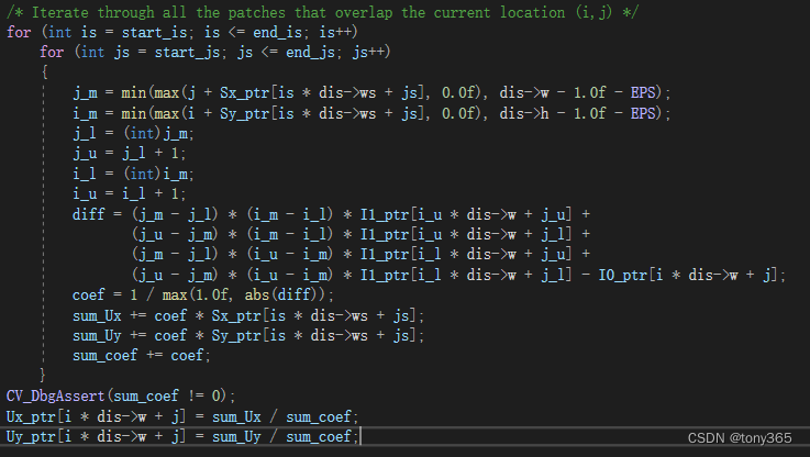
7) Densification_ParBody: patch flow fusion
在论文中有介绍融合方法:
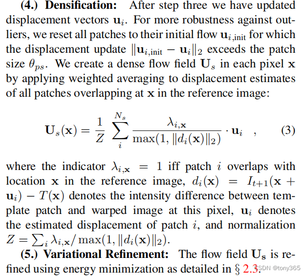
以上求得是每个patch的光流,由于patch间隔不同存在overlap的时候,就加权平均得到某个像素的flow。
就是说该像素点 被多少个patch覆盖了,就求出多少个weight,这里Us表示.weight计算根据 I1warp(p)和I0(p)的差异得到。
差异越小说明warp更可能是对的,则weight更大。
最后加权融合得到该像素点的 u和v
void DISOpticalFlowImpl::Densification_ParBody::operator()(const Range &range) const
和文中公式一致
8)最后利用变分优化方法优化u, v
if (variational_refinement_iter > 0)
    variational_refinement_processors[i]->calcUV(I0s[i], I1s[i], Ux[i], Uy[i]);
关于variational_refinement优化原理查看下一章节。
2.0 disflow中的VariationalRefinement方法
2.0 python调用code:
algo_var_refine = cv2.VariationalRefinement_create()
algo_var_refine.calcUV(im1, im2, flow_pca[..., 0].astype(np.float32), flow_pca[..., 1].astype(np.float32))
flow_var_refine = flow_pca
这是一个全局优化光流的方法,在disflow 和 deepflow中都有使用。
主要原理来自于两篇论文
论文1:High Accuracy Optical Flow Estimation Based on a
Theory for Warping[2004]
和
论文2:Beyond Pixels: Exploring New Representations and
Applications for Motion Analysis中的 A和B章节
2.1 光流变分模型
a. 灰度光流约束:
I ( x , y , t ) = I ( x + u , y + v , t + 1 ) I(x, y, t)=I(x+u,y+v,t+1) I(x,y,t)=I(x+u,y+v,t+1) (1)
上面公式的线性版本如下,但是下面等式成立的条件是运动是线性的:
I x u + I y u + I t = 0 I_xu+I_yu+I_t=0 Ixu+Iyu+It=0 (2)
b. 梯度光流约束
灰度可能容易受到图像亮度变化的影响,梯度会有更好的鲁棒性,因此引入梯度光流约束

最终的data项约束为:
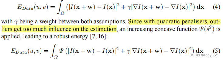
其中
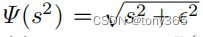
为什么用公式(5)而不是公式公式(4)?
原因是quadratic penalisers 容易收到outlier的影响
这也是二范数和一范数的区别。深度学习的损失函数也是同样的道理,如果想要损失都较小用平方L2; L1作为损失函数容易使部分sample loss=0,部分loss比较大,不受outlier的影响
c. 平滑约束
包含时域平滑和空域平滑,如果只有前后两帧则只包括空域平滑, 公式如下:


表示的x方向,y方向,时间t方向的偏微分(梯度),如果只有两张图像,就只剩下x方向和y方向。(最少3张图才能构成两张 时域上的梯度图,才能建立约束。)
d. 最终的约束方程:
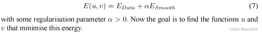
约束方程是关于两个函数u(x,y), v(x,y)的泛函。
在论文1中利用变分法求解, 转化为欧拉-拉格朗日方程后,利用fixed point iteration
loop 求解,论文1和2分别采用变分法和IterativeReweightedLeastSquare求解。因为opencv中的VariationalRefinement和论文2比较一致且论文2易懂,下面主要介绍论文2的求解方法。
2.2 优化求解
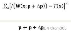
以下面的优化目标为例:

为什么选择下面的惩罚函数,原理已经说过,是为例避免outlier的影响。
少了一个梯度项,不过优化原理是一样的。
在迭代框架下,可以改为:
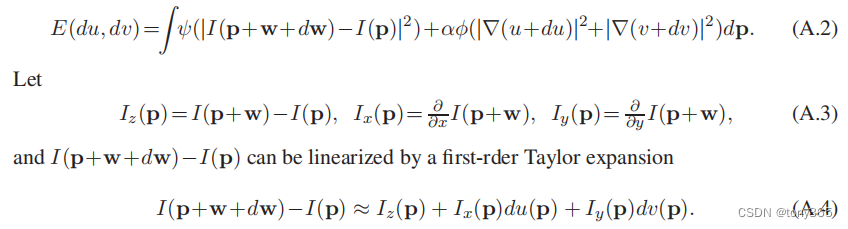
这里主要使用了一阶泰勒展开。
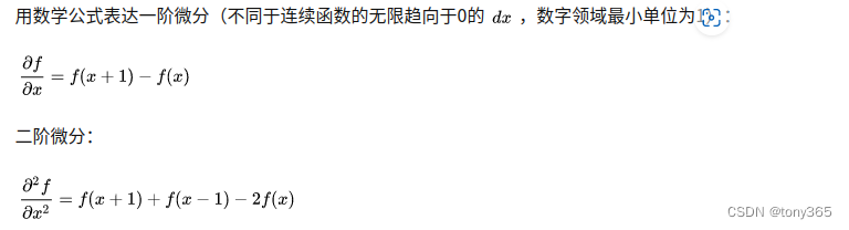
设 u + d u u+du u+du在x和y方向上的梯度为 ( u + d u ) x (u+du)_x (u+du)x和 ( u + d u ) y (u+du)_y (u+du)y,等价与
D x = [ − 1 , 0 , 1 ] Dx=[-1,0,1] Dx=[−1,0,1]算子,
D y = D x T Dy=Dx^T Dy=DxT算子
做卷积。
令 f = ( I z + I x d u + I y d v ) 2 f=(I_z+I_xdu+I_ydv)^2 f=(Iz+Ixdu+Iydv)2
g = ( D x ∗ ( u + d u ) ) 2 + ( D y ∗ ( u + d u ) ) 2 + ( D x ∗ ( v + d v ) ) 2 + ( D y ∗ ( v + d v ) ) 2 g=(Dx*(u+du))^2+(Dy*(u+du))^2+(Dx*(v+dv))^2+(Dy*(v+dv))^2 g=(Dx∗(u+du))2+(Dy∗(u+du))2+(Dx∗(v+dv))2+(Dy∗(v+dv))2
∗ * ∗号卷积,表示求偏导。
则可以得到:
E ( d u , d v ) = ∑ ( φ ( f ) + α ϕ ( g ) ) = ∑ ( φ ( ( I z + I x d u + I y d v ) 2 ) + α ϕ ( ( D x ∗ ( u + d u ) ) 2 + ( D y ∗ ( u + d u ) ) 2 + ( D x ∗ ( v + d v ) ) 2 + ( D y ∗ ( v + d v ) ) 2 ) ) E(du,dv)=\sum(\varphi(f) + \alpha\phi(g))\\ =\sum(\varphi((I_z+I_xdu+I_ydv)^2) + \alpha\phi((Dx*(u+du))^2+(Dy*(u+du))^2+(Dx*(v+dv))^2+(Dy*(v+dv))^2)) E(du,dv)=∑(φ(f)+αϕ(g))=∑(φ((Iz+Ixdu+Iydv)2)+αϕ((Dx∗(u+du))2+(Dy∗(u+du))2+(Dx∗(v+dv))2+(Dy∗(v+dv))2))
求和符合表示所有pixel.
iterative reweighted least squares (IRLS) 利用
gradient = 0求解 du, dv
∂ E ( d u , d v ) ∂ d u = 0 \frac{\partial E(du,dv)}{\partial du}=0 ∂du∂E(du,dv)=0
∂ E ( d u , d v ) ∂ d v = 0 \frac{\partial E(du,dv)}{\partial dv}=0 ∂dv∂E(du,dv)=0
∂ E ( d u , d v ) ∂ d u = ∑ 2 ( φ ′ ( f ) ( I z + I x d u + I y d v ) I x + α ϕ ′ ( g ) ( ( D x ∗ ( u + d u ) ∗ D x ) + ( D y ∗ ( u + d u ) ∗ D y ) ) ) = ∑ 2 ( φ ′ ( ( I z + I x d u + I y d v ) 2 ) ( I z + I x d u + I y d v ) I x + α ϕ ′ ( g ) ( ( D x ∗ ( u + d u ) ∗ D x ) + ( D x ∗ ( u + d u ) ∗ D x ) ) ) = ∑ 2 ( φ ′ ( ( I z + I x d u + I y d v ) 2 ) ( I z + I x d u + I y d v ) I x + α ( ( D x D x ∗ ϕ ′ ( g ) + ( D y D y ∗ ϕ ′ ( g ) ) ( u + d u ) ) \frac{\partial E(du,dv)}{\partial du}\\ =\sum2(\varphi'(f)(I_z+I_xdu+I_ydv)I_x + \alpha\phi'(g)((Dx*(u+du)*Dx)+(Dy*(u+du)*Dy)))\\ =\sum2(\varphi'((I_z+I_xdu+I_ydv)^2)(I_z+I_xdu+I_ydv)I_x + \alpha\phi'(g)((Dx*(u+du)*Dx)+(Dx*(u+du)*Dx)))\\ =\sum2(\varphi'((I_z+I_xdu+I_ydv)^2)(I_z+I_xdu+I_ydv)I_x + \alpha((DxDx*\phi'(g)+(DyDy*\phi'(g))(u+du)) ∂du∂E(du,dv)=∑2(φ′(f)(Iz+Ixdu+Iydv)Ix+αϕ′(g)((Dx∗(u+du)∗Dx)+(Dy∗(u+du)∗Dy)))=∑2(φ′((Iz+Ixdu+Iydv)2)(Iz+Ixdu+Iydv)Ix+αϕ′(g)((Dx∗(u+du)∗Dx)+(Dx∗(u+du)∗Dx)))=∑2(φ′((Iz+Ixdu+Iydv)2)(Iz+Ixdu+Iydv)Ix+α((DxDx∗ϕ′(g)+(DyDy∗ϕ′(g))(u+du))
两个一阶导近似一个空间二阶导数 拉普拉斯算子
令 L = D x D x ∗ ϕ ′ ( g ) + D y D y ∗ ϕ ′ ( g ) L=DxDx*\phi'(g)+DyDy*\phi'(g) L=DxDx∗ϕ′(g)+DyDy∗ϕ′(g)
迭代计算的时候 f f f 也可以用warp后的图像 的平方表示,
因此首先初始化 du=dv=0,
然后计算 f f f和 g g g
然后计算 φ ′ ( f ) \varphi'(f) φ′(f), ϕ ′ ( g ) \phi'(g) ϕ′(g), L
∂ E ( d u , d v ) ∂ d u = 2 ∑ ( φ ′ ( f ) I x 2 + α L ) d u + φ ′ ( f ) I x I y d v + φ ′ ( f ) I x I z + α L u \frac{\partial E(du,dv)}{\partial du}=2\sum{(\varphi'(f)I_x^2 + \alpha L) du + \varphi'(f)I_x I_y dv + \varphi'(f)I_x I_z + \alpha L u} ∂du∂E(du,dv)=2∑(φ′(f)Ix2+αL)du+φ′(f)IxIydv+φ′(f)IxIz+αLu
同理:
∂ E ( d u , d v ) ∂ d v = 2 ∑ ( φ ′ ( f ) I y 2 + α L ) d v + φ ′ ( f ) I x I y d u + φ ′ ( f ) I y I z + α L v \frac{\partial E(du,dv)}{\partial dv}=2\sum{(\varphi'(f)I_y^2 + \alpha L) dv + \varphi'(f)I_x I_y du + \varphi'(f)I_y I_z + \alpha L v} ∂dv∂E(du,dv)=2∑(φ′(f)Iy2+αL)dv+φ′(f)IxIydu+φ′(f)IyIz+αLv
令 ∂ E ( d u , d v ) ∂ d u = 0 \frac{\partial E(du,dv)}{\partial du}=0 ∂du∂E(du,dv)=0和 ∂ E ( d u , d v ) ∂ d v = 0 \frac{\partial E(du,dv)}{\partial dv}=0 ∂dv∂E(du,dv)=0
得到:
Ax = b
其中
A= [ ( φ ′ ( f ) I x 2 + α L ) φ ′ ( f ) I x I y φ ′ ( f ) I x I y φ ′ ( f ) I y 2 + α L ) ] \begin{bmatrix} (\varphi'(f)I_x^2 + \alpha L) & \varphi'(f)I_x I_y \\ \varphi'(f)I_x I_y & \varphi'(f)I_y^2 + \alpha L) \end{bmatrix} [(φ′(f)Ix2+αL)φ′(f)IxIyφ′(f)IxIyφ′(f)Iy2+αL)]
x = [ d u d v ] \begin{bmatrix} du \\ dv \end{bmatrix} [dudv]
b= − [ φ ′ ( f ) I x I z + α L u φ ′ ( f ) I y I z + α L v ] -\begin{bmatrix} \varphi'(f)I_x I_z + \alpha L u \\ \varphi'(f)I_y I_z + \alpha L v \end{bmatrix} −[φ′(f)IxIz+αLuφ′(f)IyIz+αLv]
因此每次迭代求解du,dv。
2.3 来看opencv的实现
主要公式就是上面的Ax = b
a. 接口类和实现类
首先接口
#include "opencv2/opencv.hpp"

using namespace std;
using namespace cv;
/** @brief Variational optical flow refinement

This class implements variational refinement of the input flow field, i.e.
it uses input flow to initialize the minimization of the following functional:
\f$E(U) = \int_{\Omega} \delta \Psi(E_I) + \gamma \Psi(E_G) + \alpha \Psi(E_S) \f$,
where \f$E_I,E_G,E_S\f$ are color constancy, gradient constancy and smoothness terms
respectively. \f$\Psi(s^2)=\sqrt{s^2+\epsilon^2}\f$ is a robust penalizer to limit the
influence of outliers. A complete formulation and a description of the minimization
procedure can be found in @cite Brox2004
*/
//主要函数就是calcUV
class VariationalRefinement
{
public:
    /** @brief @ref calc function overload to handle separate horizontal (u) and vertical (v) flow components
    (to avoid extra splits/merges) */
    virtual void calcUV(InputArray I0, InputArray I1, InputOutputArray flow_u, InputOutputArray flow_v) = 0;

    /** @brief Number of outer (fixed-point) iterations in the minimization procedure.
    @see setFixedPointIterations */
    virtual int getFixedPointIterations() const = 0;
    /** @copybrief getFixedPointIterations @see getFixedPointIterations */
    virtual void setFixedPointIterations(int val) = 0;

    /** @brief Number of inner successive over-relaxation (SOR) iterations
        in the minimization procedure to solve the respective linear system.
    @see setSorIterations */
    virtual int getSorIterations() const = 0;
    /** @copybrief getSorIterations @see getSorIterations */
    virtual void setSorIterations(int val) = 0;

    /** @brief Relaxation factor in SOR
    @see setOmega */
    virtual float getOmega() const = 0;
    /** @copybrief getOmega @see getOmega */
    virtual void setOmega(float val) = 0;

    /** @brief Weight of the smoothness term
    @see setAlpha */
    virtual float getAlpha() const = 0;
    /** @copybrief getAlpha @see getAlpha */
    virtual void setAlpha(float val) = 0;

    /** @brief Weight of the color constancy term
    @see setDelta */
    virtual float getDelta() const = 0;
    /** @copybrief getDelta @see getDelta */
    virtual void setDelta(float val) = 0;

    /** @brief Weight of the gradient constancy term
    @see setGamma */
    virtual float getGamma() const = 0;
    /** @copybrief getGamma @see getGamma */
    virtual void setGamma(float val) = 0;

    /** @brief Creates an instance of VariationalRefinement
    */
    static Ptr<VariationalRefinement> create();
};
实现类:
class VariationalRefinementImpl
{
public:
    VariationalRefinementImpl();

    void calc(InputArray I0, InputArray I1, InputOutputArray flow) ;
    void calcUV(InputArray I0, InputArray I1, InputOutputArray flow_u, InputOutputArray flow_v)  ;
    void collectGarbage()  ;

protected: //!< algorithm parameters
    int fixedPointIterations, sorIterations;
    float omega;
    float alpha, delta, gamma;
    float zeta, epsilon;

public:
    int getFixedPointIterations() const   { return fixedPointIterations; }
    void setFixedPointIterations(int val)   { fixedPointIterations = val; }
    int getSorIterations() const   { return sorIterations; }
    void setSorIterations(int val)   { sorIterations = val; }
    float getOmega() const   { return omega; }
    void setOmega(float val)   { omega = val; }
    float getAlpha() const   { return alpha; }
    void setAlpha(float val)   { alpha = val; }
    float getDelta() const   { return delta; }
    void setDelta(float val)   { delta = val; }
    float getGamma() const   { return gamma; }
    void setGamma(float val)   { gamma = val; }

protected: //!< internal buffers
  /* This struct defines a special data layout for Mat_<float>. Original buffer is split into two: one for "red"
   * elements (sum of indices is even) and one for "black" (sum of indices is odd) in a checkerboard pattern. It
   * allows for more efficient processing in SOR iterations, more natural SIMD vectorization and parallelization
   * (Red-Black SOR). Additionally, it simplifies border handling by adding repeated borders to both red and
   * black buffers.
   */
    struct RedBlackBuffer
    {
        Mat_<float> red;   //!< (i+j)%2==0
        Mat_<float> black; //!< (i+j)%2==1

        /* Width of even and odd rows may be different */
        int red_even_len, red_odd_len;
        int black_even_len, black_odd_len;

        RedBlackBuffer();
        void create(Size s);
        void release();
    };

    Mat_<float> Ix, Iy, Iz, Ixx, Ixy, Iyy, Ixz, Iyz;                            //!< image derivative buffers
    RedBlackBuffer Ix_rb, Iy_rb, Iz_rb, Ixx_rb, Ixy_rb, Iyy_rb, Ixz_rb, Iyz_rb; //!< corresponding red-black buffers

    RedBlackBuffer A11, A12, A22, b1, b2; //!< main linear system coefficients
    RedBlackBuffer weights;               //!< smoothness term weights in the current fixed point iteration

    Mat_<float> mapX, mapY; //!< auxiliary buffers for remapping

    RedBlackBuffer tempW_u, tempW_v; //!< flow buffers that are modified in each fixed point iteration
    RedBlackBuffer dW_u, dW_v;       //!< optical flow increment
    RedBlackBuffer W_u_rb, W_v_rb;   //!< red-black-buffer version of the input flow

private: //!< private methods and parallel sections
    void splitCheckerboard(RedBlackBuffer& dst, Mat& src);
    void mergeCheckerboard(Mat& dst, RedBlackBuffer& src);
    void updateRepeatedBorders(RedBlackBuffer& dst);
    void warpImage(Mat& dst, Mat& src, Mat& flow_u, Mat& flow_v);
    void prepareBuffers(Mat& I0, Mat& I1, Mat& W_u, Mat& W_v);

    /* Parallelizing arbitrary operations with 3 input/output arguments */
    typedef void (VariationalRefinementImpl::* Op)(void* op1, void* op2, void* op3);
    struct ParallelOp_ParBody : public ParallelLoopBody
    {
        VariationalRefinementImpl* var;
        vector<Op> ops;
        vector<void*> op1s;
        vector<void*> op2s;
        vector<void*> op3s;

        ParallelOp_ParBody(VariationalRefinementImpl& _var, vector<Op> _ops, vector<void*>& _op1s,
            vector<void*>& _op2s, vector<void*>& _op3s);
        void operator()(const Range& range) const  ;
    };
    void gradHorizAndSplitOp(void* src, void* dst, void* dst_split)
    {


        Sobel(*(Mat*)src, *(Mat*)dst, -1, 1, 0, 1, 1, 0.00, BORDER_REPLICATE);
        splitCheckerboard(*(RedBlackBuffer*)dst_split, *(Mat*)dst);
    }
    void gradVertAndSplitOp(void* src, void* dst, void* dst_split)
    {


        Sobel(*(Mat*)src, *(Mat*)dst, -1, 0, 1, 1, 1, 0.00, BORDER_REPLICATE);
        splitCheckerboard(*(RedBlackBuffer*)dst_split, *(Mat*)dst);
    }
    void averageOp(void* src1, void* src2, void* dst)
    {


        addWeighted(*(Mat*)src1, 0.5, *(Mat*)src2, 0.5, 0.0, *(Mat*)dst, CV_32F);
    }
    void subtractOp(void* src1, void* src2, void* dst)
    {


        subtract(*(Mat*)src1, *(Mat*)src2, *(Mat*)dst, noArray(), CV_32F);
    }

    struct ComputeDataTerm_ParBody : public ParallelLoopBody
    {
        VariationalRefinementImpl* var;
        int nstripes, stripe_sz;
        int h;
        RedBlackBuffer* dW_u, * dW_v;
        bool red_pass;

        ComputeDataTerm_ParBody(VariationalRefinementImpl& _var, int _nstripes, int _h, RedBlackBuffer& _dW_u,
            RedBlackBuffer& _dW_v, bool _red_pass);
        void operator()(const Range& range) const  ;
    };

    struct ComputeSmoothnessTermHorPass_ParBody : public ParallelLoopBody
    {
        VariationalRefinementImpl* var;
        int nstripes, stripe_sz;
        int h;
        RedBlackBuffer* W_u, * W_v, * curW_u, * curW_v;
        bool red_pass;

        ComputeSmoothnessTermHorPass_ParBody(VariationalRefinementImpl& _var, int _nstripes, int _h,
            RedBlackBuffer& _W_u, RedBlackBuffer& _W_v, RedBlackBuffer& _tempW_u,
            RedBlackBuffer& _tempW_v, bool _red_pass);
        void operator()(const Range& range) const  ;
    };

    struct ComputeSmoothnessTermVertPass_ParBody : public ParallelLoopBody
    {
        VariationalRefinementImpl* var;
        int nstripes, stripe_sz;
        int h;
        RedBlackBuffer* W_u, * W_v;
        bool red_pass;

        ComputeSmoothnessTermVertPass_ParBody(VariationalRefinementImpl& _var, int _nstripes, int _h,
            RedBlackBuffer& W_u, RedBlackBuffer& _W_v, bool _red_pass);
        void operator()(const Range& range) const  ;
    };

    struct RedBlackSOR_ParBody : public ParallelLoopBody
    {
        VariationalRefinementImpl* var;
        int nstripes, stripe_sz;
        int h;
        RedBlackBuffer* dW_u, * dW_v;
        bool red_pass;

        RedBlackSOR_ParBody(VariationalRefinementImpl& _var, int _nstripes, int _h, RedBlackBuffer& _dW_u,
            RedBlackBuffer& _dW_v, bool _red_pass);
        void operator()(const Range& range) const  ;
    };
};
b. 具体实现介绍
- 上面有一些struct 继承自ParallelLoopBody, 主要是tbb的优化方法并行加速操作
- calc函数: 比如输入为I0,I1两个图像,和一个光流flow, 然后主要调用calcUV函数
void VariationalRefinementImpl::calc(InputArray I0, InputArray I1, InputOutputArray flow)
{
    CV_Assert(!I0.empty() && I0.channels() == 1);
    CV_Assert(!I1.empty() && I1.channels() == 1);
    CV_Assert(I0.sameSize(I1));
    CV_Assert((I0.depth() == CV_8U && I1.depth() == CV_8U) || (I0.depth() == CV_32F && I1.depth() == CV_32F));
    CV_Assert(!flow.empty() && flow.depth() == CV_32F && flow.channels() == 2);
    CV_Assert(I0.sameSize(flow));

    Mat uv[2];
    Mat& flowMat = flow.getMatRef();
    split(flowMat, uv);
    calcUV(I0, I1, uv[0], uv[1]);
    merge(uv, 2, flowMat);
}
- calcUV函数:也是整个算法的框架
void VariationalRefinementImpl::calcUV(InputArray I0, InputArray I1, InputOutputArray flow_u, InputOutputArray flow_v)
{

   //一些assert操作, 对输入的要求
    CV_Assert(!I0.empty() && I0.channels() == 1);
    CV_Assert(!I1.empty() && I1.channels() == 1);
    CV_Assert(I0.sameSize(I1));
    CV_Assert((I0.depth() == CV_8U && I1.depth() == CV_8U) || (I0.depth() == CV_32F && I1.depth() == CV_32F));
    CV_Assert(!flow_u.empty() && flow_u.depth() == CV_32F && flow_u.channels() == 1);
    CV_Assert(!flow_v.empty() && flow_v.depth() == CV_32F && flow_v.channels() == 1);
    CV_Assert(I0.sameSize(flow_u));
    CV_Assert(flow_u.sameSize(flow_v));

    int num_stripes = getNumThreads();//多线程相关,可以不做了解
    Mat I0Mat = I0.getMat();
    Mat I1Mat = I1.getMat();
    Mat& W_u = flow_u.getMatRef();
    Mat& W_v = flow_v.getMatRef();
    prepareBuffers(I0Mat, I1Mat, W_u, W_v);

    splitCheckerboard(W_u_rb, W_u);
    splitCheckerboard(W_v_rb, W_v);
    W_u_rb.red.copyTo(tempW_u.red);
    W_u_rb.black.copyTo(tempW_u.black);
    W_v_rb.red.copyTo(tempW_v.red);
    W_v_rb.black.copyTo(tempW_v.black);
    dW_u.red.setTo(0.0f);
    dW_u.black.setTo(0.0f);
    dW_v.red.setTo(0.0f);
    dW_v.black.setTo(0.0f);

    for (int i = 0; i < fixedPointIterations; i++)
    {
        //CV_TRACE_REGION("fixedPoint_iteration");

        parallel_for_(Range(0, num_stripes), ComputeDataTerm_ParBody(*this, num_stripes, I0Mat.rows, dW_u, dW_v, true));
        parallel_for_(Range(0, num_stripes), ComputeDataTerm_ParBody(*this, num_stripes, I0Mat.rows, dW_u, dW_v, false));

        parallel_for_(Range(0, num_stripes), ComputeSmoothnessTermHorPass_ParBody(
            *this, num_stripes, I0Mat.rows, W_u_rb, W_v_rb, tempW_u, tempW_v, true));
        parallel_for_(Range(0, num_stripes), ComputeSmoothnessTermHorPass_ParBody(
            *this, num_stripes, I0Mat.rows, W_u_rb, W_v_rb, tempW_u, tempW_v, false));

        parallel_for_(Range(0, num_stripes),
            ComputeSmoothnessTermVertPass_ParBody(*this, num_stripes, I0Mat.rows, W_u_rb, W_v_rb, true));
        parallel_for_(Range(0, num_stripes),
            ComputeSmoothnessTermVertPass_ParBody(*this, num_stripes, I0Mat.rows, W_u_rb, W_v_rb, false));

        for (int j = 0; j < sorIterations; j++)
        {
            //CV_TRACE_REGION("SOR_iteration");
            parallel_for_(Range(0, num_stripes), RedBlackSOR_ParBody(*this, num_stripes, I0Mat.rows, dW_u, dW_v, true));
            parallel_for_(Range(0, num_stripes), RedBlackSOR_ParBody(*this, num_stripes, I0Mat.rows, dW_u, dW_v, false));
        }

        tempW_u.red = W_u_rb.red + dW_u.red;
        tempW_u.black = W_u_rb.black + dW_u.black;
        updateRepeatedBorders(tempW_u);
        tempW_v.red = W_v_rb.red + dW_v.red;
        tempW_v.black = W_v_rb.black + dW_v.black;
        updateRepeatedBorders(tempW_v);
    }
    mergeCheckerboard(W_u, tempW_u);
    mergeCheckerboard(W_v, tempW_v);
}
算法框架:
1)prepareBuffers函数中warp I1得到warpedI,然后让它与 I0 求个平均(这里只是增加鲁棒性), 对应I(p+w)
主要计算
a v e r a g e d I = I 0 ∗ 0.5 + w a r p e d I ∗ 0.5 对应公式中的 I ( p + w ) I z = w a r p e d I − I 0 对应公式中的 I z I x I y I x z I y z I x x I y y I x y 都是字面意思 averagedI = I0*0.5 +warpedI*0.5 \qquad 对应公式中的 I(p+w)\\ Iz = warpedI - I0 \qquad 对应公式中的 Iz\\ Ix\\ Iy\\ Ixz\\ Iyz\\ Ixx\\ Iyy\\ Ixy \qquad 都是字面意思 averagedI=I0∗0.5+warpedI∗0.5对应公式中的I(p+w)Iz=warpedI−I0对应公式中的IzIxIyIxzIyzIxxIyyIxy都是字面意思
后缀 _rb 是把矩阵分成两个,主要是为了方便计算。
2)ComputeDataTerm_ParBody
weight 对应 φ ′ ( f ) \varphi'(f) φ′(f)
a11, a12, a22, b1,b2 都可以求出,当然这只是 gray 约束
/* Step 1: Compute color constancy terms */
/* Normalization factor:*/
derivNorm = pIx[j] * pIx[j] + pIy[j] * pIy[j] + zeta_squared;
/* Color constancy penalty (computed by Taylor expansion):*/
Ik1z = pIz[j] + pIx[j] * pdU[j] + pIy[j] * pdV[j];
/* Weight of the color constancy term in the current fixed-point iteration divided by derivNorm: */
weight = (delta2 / sqrt(Ik1z * Ik1z / derivNorm + epsilon_squared)) / derivNorm;
/* Add respective color constancy terms to the linear system coefficients: */
pa11[j] = weight * (pIx[j] * pIx[j]) + zeta_squared;
pa12[j] = weight * (pIx[j] * pIy[j]);
pa22[j] = weight * (pIy[j] * pIy[j]) + zeta_squared;
pb1[j] = -weight * (pIz[j] * pIx[j]);
pb2[j] = -weight * (pIz[j] * pIy[j]);
代码中同样计算了 gradiant 约束。
3)ComputeSmoothnessTermHorPass_ParBody 和 ComputeSmoothnessTermVertPass_ParBody
计算水平和竖直方向上的平滑约束
pWeight[j] = alpha2 / sqrt(ux * ux + vx * vx + uy * uy + vy * vy + epsilon_squared); 这里求 ϕ \phi ϕ的导数,对应 α ϕ ′ ( g ) \alpha \phi'(g) αϕ′(g)
经过以上步骤后得到 A 和 b,然后求x.
4) RedBlackSOR_ParBody
solve Ax = b
sigmaU = pW_next[j - 1] * pdu_next[j - 1] + pW[j] * pdu_next[j] + pW_prev_row[j] * pdu_prev_row[j] + pW[j] * pdu_next_row[j];
sigmaV = pW_next[j - 1] * pdv_next[j - 1] + pW[j] * pdv_next[j] + pW_prev_row[j] * pdv_prev_row[j] +pW[j] * pdv_next_row[j];
pdu[j] += var->omega * ((sigmaU + pb1[j] - pdv[j] * pa12[j]) / pa11[j] - pdu[j]);
pdv[j] += var->omega * ((sigmaV + pb2[j] - pdu[j] * pa12[j]) / pa22[j] - pdv[j]);
参考:
Large Displacement Optical Flow: Descriptor Matching in Variational Motion Estimation
对上面的方法进行优化,增加匹配项约束,意思就是加入我们检测数一些特征点匹配,这些匹配点可以得到 u,v, 增加约束。
图像处理中的全局优化技术(Global optimization techniques in image processing and computer vision) (三) 介绍了几篇 变分光流法论文
3 线性方程组解法
关于线性方程组的数值解法一般有两类:直接法和迭代法
- 直接法:直接法就是经过有限步算术运算,可求得线性方程组精确解的方法(若计算过程中没有舍入误差)。常用于求解低阶稠密矩阵方程组及某些大型稀疏矩阵方程组(如大型带状方程组)。
- 迭代法:迭代法就是用某种极限过程去逐步逼近线性方程组精确解的方法。优点:存储单元少、程序设计简单、原始系数矩阵在计算过程始终不变等;缺点:存在收敛性及收敛速度问题。常用于求解大型稀疏矩阵方程组(尤其是由微分方程离散后得到的大型方程组)。
直接法的介绍参考:第5章 解线性方程组的直接方法
迭代法参考:第6章 解线性方程组的迭代法(基于MATLAB)
解线性方程组的迭代法
数值分析】Jacobi、Seidel和Sor迭代法求解线性方程组(附matlab代码)
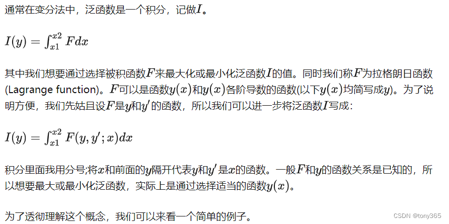
4 变分法
定义:泛函是以函数为变量的函数。即它的输入是函数,输出是实数。而这个输出值取决于一个或多个函数(输入)在一整个路径上的积分。
那么什么是变分法呢?求泛函极值的方法称为变分法。
变分法将泛函极值问题转换为一个非线性偏微分方程,又称为PDE,怎么求这个方程呢?
一般是转化为非线性代数方程组,然后迭代的方法求解,比如梯度下降。
应用在图像降噪和修复,dense flow estimation等。
变分法简介Part 1.(Calculus of Variations) 该系列有系统的介绍
浅谈变分原理
详细的示例
基于变分法的感知色彩校正 这是一个特别好的应用
5 参考文献
关于Lucas-Kanade 光流法原理:
-
Lucas-Kanade 20 Years On: A Unifying Framework 翻译(一)
讲解了1)光流法模型,2)warp方式, 3)inverse search方法。4)耗时
很有参考价值,比如
不同的warp方式的优化。不是optical flow这种直接相加的warp,而是仿射变换的参数化 warp, 也可以求出仿射变换的参数。只不过每个点都有自己的仿射参数。换句话说,加入两幅图像满足仿射变换关系,可以通过这个方法来求解变换关系,应用在前后帧的对齐上。
-
视觉SLAM十四讲作业练习(6) 光流法跟踪单点,有代码。
-
DIS 光流详解 对Fast Optical Flow using Dense Inverse Search论文的概述
关于DIS代码:
- of_dis
- Optical flow using dense inverse search
- opencv代码:opencv4以上版本 在 video/tracking 模块中, 还是opencv清晰易读一些
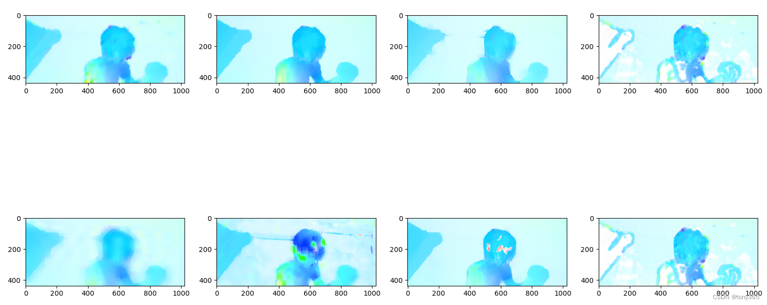
6 python 光流实验:
利用MPI-Sintel的一组图片,调用各种光流方法:
import os
import cv2
import numpy as np
from matplotlib import pyplot as plt
from matplotlib.colors import hsv_to_rgb
from torchvision.utils import flow_to_image
import torch
from show_flow import draw_flow
import time

def flow_to_image_torch(flow):
    flow = torch.from_numpy(np.transpose(flow, [2, 0, 1]))
    flow_im = flow_to_image(flow)
    img = np.transpose(flow_im.numpy(), [1, 2, 0])
    #print(img.shape)
    return img

def show_flow_im(frame, flow):
    h, w, c = frame.shape
    flow_im3 = flow_to_image_torch(flow)
    #print(h, w, c, min(h, w)//40)
    flow_im4 = draw_flow(frame, flow, 20)
    plt.figure()
    plt.subplot(121)
    plt.imshow(flow_im3)
    plt.subplot(122)
    plt.imshow(flow_im4)
    plt.show()

def cal_flow(frame1, frame2):
    """
    :param frame1: input image 1
    :param frame2: input image 2
    :return: optical flow
    """
    im1 = cv2.cvtColor(frame1, cv2.COLOR_BGR2GRAY)
    im2 = cv2.cvtColor(frame2, cv2.COLOR_BGR2GRAY)

    algo_dis = cv2.DISOpticalFlow_create(cv2.DISOPTICAL_FLOW_PRESET_MEDIUM)
    algo_dis.setUseSpatialPropagation(True)
    flow = algo_dis.calc(im1, im2, None, )

    return flow
def cal_flow_algos(frame1, frame2):
    """
    :param frame1: input image 1
    :param frame2: input image 2
    :return: optical flow
    """
    im1 = cv2.cvtColor(frame1, cv2.COLOR_BGR2GRAY)
    im2 = cv2.cvtColor(frame2, cv2.COLOR_BGR2GRAY)
    times = []
    start = time.time()
    algo_dis = cv2.DISOpticalFlow_create(cv2.DISOPTICAL_FLOW_PRESET_MEDIUM)
    algo_dis.setUseSpatialPropagation(True)
    flow_dis = algo_dis.calc(im1, im2, None, )
    end = time.time()
    times.append(end-start)

    start = end
    algo_deepflow = cv2.optflow.createOptFlow_DeepFlow()
    flow_deepflow = algo_deepflow.calc(im1, im2, None)
    end = time.time()
    times.append(end-start)

    start = end
    flow_sparse = cv2.optflow.calcOpticalFlowSparseToDense(im1, im2)
    end = time.time()
    times.append(end - start)

    start = end
    flow_fb = cv2.calcOpticalFlowFarneback(im1, im2, None, 0.5, 3, 15, 3, 5, 1.2, 0)
    end = time.time()
    times.append(end - start)

    start = end
    algo_pca = cv2.optflow.createOptFlow_PCAFlow()
    flow_pca = algo_pca.calc(im1, im2, None)
    end = time.time()
    times.append(end - start)

    start = end
    flow_simple = cv2.optflow.calcOpticalFlowSF(frame1, frame2, 1, 5, 5) # color image
    end = time.time()
    times.append(end - start)

    start = end
    flow_TVL1 = cv2.optflow.DualTVL1OpticalFlow_create()
    flow_tvl1 = flow_TVL1.calc(im1, im2, None)
    end = time.time()
    times.append(end - start)

    start = end
    algo_var_refine = cv2.VariationalRefinement_create()
    flow_var_refine = flow_fb
    algo_var_refine.calcUV(im1, im2, flow_var_refine[..., 0].astype(np.float32), flow_var_refine[..., 1].astype(np.float32))

    end = time.time()
    times.append(end - start)
    print(flow_var_refine.shape)
    print('run time:', times)
    return [flow_dis, flow_deepflow, flow_sparse, flow_fb, flow_pca, flow_simple, flow_tvl1, flow_var_refine]

def flow_warp(im1, im2, flow):
    """
    :param im1: pre image
    :param im2: next image
    :param flow: optical flow ,im1 to im2
    :return:
    """
    h, w, c = im1.shape
    hh = np.arange(0, h)
    ww = np.arange(0, w)
    xx, yy = np.meshgrid(ww, hh)

    tx = xx - flow[..., 0]
    ty = yy - flow[..., 1]
    mask = ((tx < 0) + (ty < 0) + (tx > w - 1) + (ty > h - 1)) > 0
    # print(mask.shape, mask.dtype, np.sum(mask))
    # out = interp_linear(image, tx, ty)
    # warped im1, should compare with im2
    out = cv2.remap(im1, tx.astype(np.float32), ty.astype(np.float32), interpolation=cv2.INTER_LINEAR)
    out[mask] = 0
    return out

def cal_epe(flow_gt, flow):
    diff = flow_gt - flow
    return np.mean(np.sqrt((np.sum(diff*diff, axis=-1))))

def load_flow_to_numpy(path):
    with open(path, 'rb') as f:
        magic = np.fromfile(f, np.float32, count=1)
        assert (202021.25 == magic), 'Magic number incorrect. Invalid .flo file'
        w = np.fromfile(f, np.int32, count=1)[0]
        h = np.fromfile(f, np.int32, count=1)[0]
        data = np.fromfile(f, np.float32, count=2 * w * h)
    data2D = np.reshape(data, (h, w, 2))
    #print(data2D[:10,:10,0])
    return data2D


if __name__ == "__main__":
    print('cv2 version: {}'.format(cv2.__version__))

    file1 = r'D:\codeflow\MPI-Sintel-complete\training\final\alley_1\frame_0001.png'
    file2 = r'D:\codeflow\MPI-Sintel-complete\training\final\alley_1\frame_0002.png'
    # 读取图片
    frame1 = cv2.imread(file1)
    h, w, c = frame1.shape

    frame2 = cv2.imread(file2)
    frame2 = cv2.resize(frame2, (w, h))

    im1 = cv2.cvtColor(frame1, cv2.COLOR_BGR2GRAY)
    im2 = cv2.cvtColor(frame2, cv2.COLOR_BGR2GRAY)

    algo_names = ['flow_dis', 'flow_deepflow', 'flow_sparse', 'flow_fb', 'flow_pca', 'flow_simple', 'flow_tvl1', 'flow_var_refine']
    # 计算光流
    flows = cal_flow_algos(frame1, frame2)

    # 读取flow gt
    file_flow = r'D:\codeflow\MPI-Sintel-complete\training\flow\alley_1\frame_0001.flo'
    flow_gt = load_flow_to_numpy(file_flow)
    flow_gt_im = flow_to_image_torch(flow_gt)
    # 计算epe
    flow_gt = cv2.resize(flow_gt, (w, h))
    epes = []
    for flow in flows:
        epe = cal_epe(flow_gt, flow)
        epes.append(epe)
    print(epes)
    # 画出光流图
    plt.figure()
    num = len(flows)
    col_num = (num + 1) // 2
    for i in range(num):
        print(flows[i].min(), flows[i].max(), flows[i].dtype, flows[i].shape)
        flows[i][np.isnan(flows[i])] = 0
        plt.subplot(2, col_num, i + 1)
        flow_im = flow_to_image_torch(flows[i])
        plt.imshow(flow_im)
        # warp
        im_warp = flow_warp(frame1, frame2, flows[i])
        # cv2.imwrite(file1[:-4]+algo_names[i]+'.png', im_warp)
    plt.show()