可解释机器学习笔记之CAM+Captum代码实战

文章目录

可解释机器学习笔记之CAM+Captum代码实战

首先非常感谢同济子豪兄拍摄的可解释机器学习公开课，并且免费分享，这门课程，包含人工智能可解释性、显著性分析领域的导论、算法综述、经典论文精读、代码实战、前沿讲座。由B站知名人工智能科普UP主“同济子豪兄”主讲。课程主页： https://github.com/TommyZihao/zihao_course/blob/main/XAI 一起打开AI的黑盒子，洞悉AI的脑回路和注意力，解释它、了解它、改进它，进而信赖它。知其然，也知其所以然。这里给出链接，倡导大家一起学习， 别忘了给子豪兄点个关注哦。

学习GitHub 内容链接：
https://github.com/TommyZihao/zihao_course/tree/main/XAI

B站视频合集链接：
https://space.bilibili.com/1900783/channel/collectiondetail?sid=713364

代码实战介绍

在前面经过4个知识的学习之后，已经对可解释机器学习有了一定的了解，但是这些有什么用呢，最重要的当然是代码实战，所以这一部分学习的就是CAM和Captum的一些可视化的代码实战，能将理论和代码结合起来，方便我们理解和学习。

所有的代码都已经分享，都在子豪兄的Github中，这是代码的Github:https://github.com/TommyZihao/Train_Custom_Dataset，可以用pytorch训练自己的图像分类模型，基于torch-cam实现各个类别、单张图像、视频文件、摄像头实时画面的CAM可视化

torch-cam工具包

这里介绍一些主要的一些可视化的用法，具体的操作和方法，在视频和代码中都有体现

可视化CAM类激活热力图

预训练ImageNet-1000图像分类-单张图像

首先可以可视化出我们的类激活图

activation_map = cam_extractor(pred_id, pred_logits)
activation_map = activation_map[0][0].detach().cpu().numpy()
plt.imshow(activation_map)
plt.show()

png

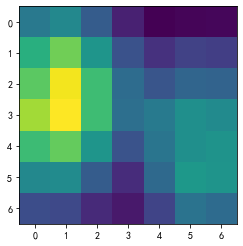
后续根据类激活图，和原有的图片进行叠加，就能得到最后的图片

from torchcam.utils import overlay_mask

result = overlay_mask(img_pil, Image.fromarray(activation_map), alpha=0.7)
result

[外链图片转存失败,源站可能有防盗链机制,建议将图片保存下来直接上传(img-0OIPlknr-1671639191799)(https://relph1119.github.io/my-team-learning/Interpretable_machine_learning44/task05/output_20_0.png)]

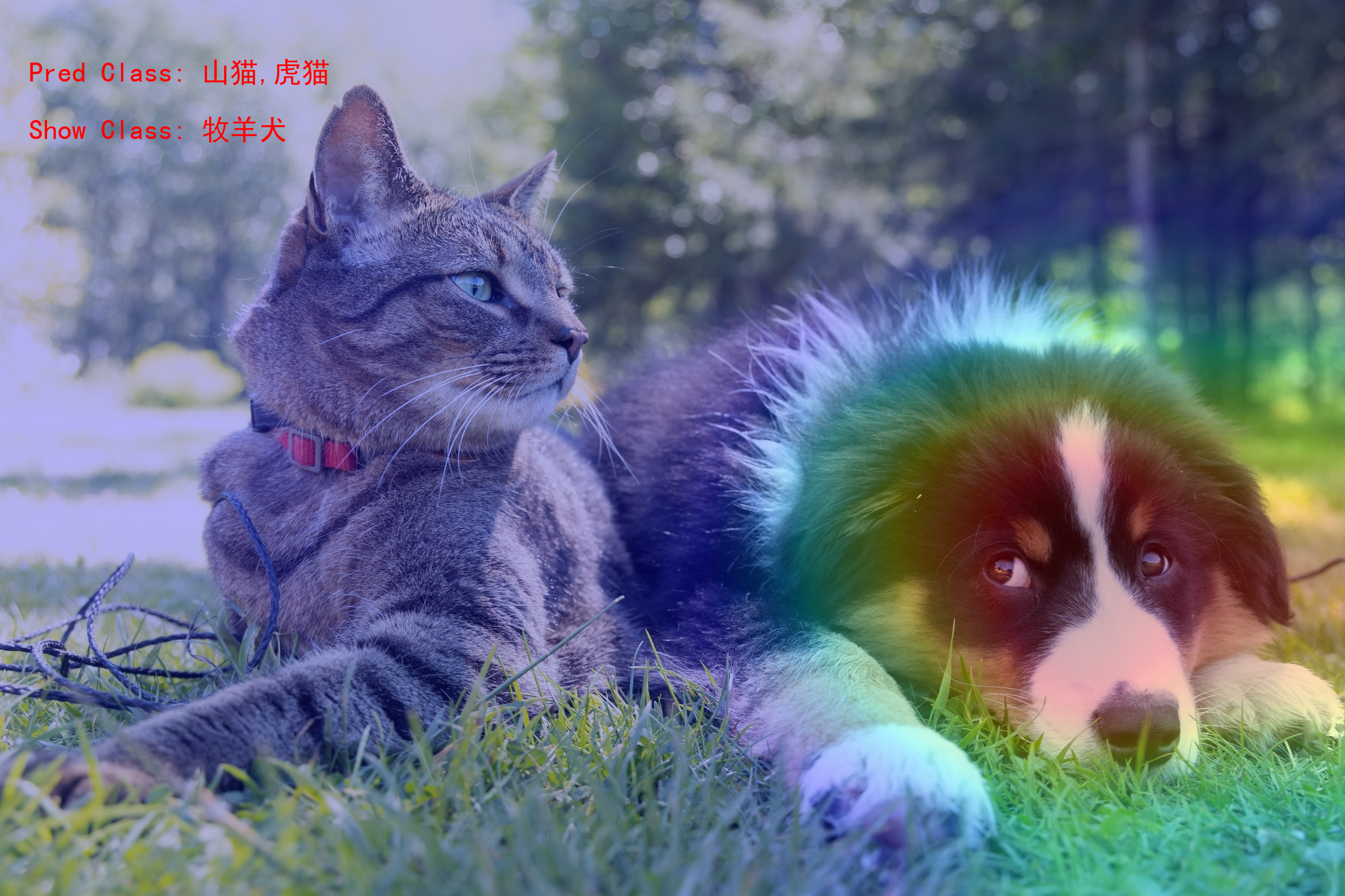
除此之外，我们还能固定可视化的类别，这样就可以展示出来我们想要的类别了。

img_path = './test_img/cat_dog.jpg'
# 可视化热力图的类别ID，如果为 None，则为置信度最高的预测类别ID

# 边牧犬
show_class_id = 231

# 是否显示中文类别
Chinese = True

def get_cam(img_pil, test_transform, model, cam_extractor, 
            show_class_id, pred_id, device):
    # 前向预测
    input_tensor = test_transform(img_pil).unsqueeze(0).to(device) # 预处理
    pred_logits = model(input_tensor)
    pred_top1 = torch.topk(pred_logits, 1)
    pred_id = pred_top1[1].detach().cpu().numpy().squeeze().item()
    
    # 可视化热力图的类别ID，如果不指定，则为置信度最高的预测类别ID
    if show_class_id:
        show_id = show_class_id
    else:
        show_id = pred_id
        show_class_id = pred_id
    
    # 生成可解释性分析热力图
    activation_map = cam_extractor(show_id, pred_logits)
    activation_map = activation_map[0][0].detach().cpu().numpy()
    result = overlay_mask(img_pil, Image.fromarray(activation_map), alpha=0.7)
    return result, pred_id, show_class_idCopy to clipboardErrorCopied

img_pil = Image.open(img_path)
result, pred_id, show_class_id = get_cam(img_pil, test_transform, model, cam_extractor, 
                                show_class_id, pred_id, device)

def print_image_label(result, pred_id, show_class_id, 
                      idx_to_labels, idx_to_labels_cn=None, Chinese=False):
    # 在图像上写字
    draw = ImageDraw.Draw(result)

    if Chinese:
        # 在图像上写中文
        text_pred = 'Pred Class: {}'.format(idx_to_labels_cn[pred_id])
        text_show = 'Show Class: {}'.format(idx_to_labels_cn[show_class_id])
    else:
        # 在图像上写英文
        text_pred = 'Pred Class: {}'.format(idx_to_labels[pred_id])
        text_show = 'Show Class: {}'.format(idx_to_labels[show_class_id])
    # 文字坐标，中文字符串，字体，rgba颜色
    draw.text((50, 100), text_pred, font=font, fill=(255, 0, 0, 1))
    draw.text((50, 200), text_show, font=font, fill=(255, 0, 0, 1))
    
    return result

result = print_image_label(result, pred_id, show_class_id,
                           idx_to_labels, idx_to_labels_cn, Chinese)
result

[外链图片转存失败,源站可能有防盗链机制,建议将图片保存下来直接上传(img-8ZGXtE9O-1671639191800)(https://relph1119.github.io/my-team-learning/Interpretable_machine_learning44/task05/output_27_0.png)]

视频以及摄像头预测

除此之外，我们还可以检测视频或者是摄像头，实际上就是一帧一帧的图片而已，原理是一样的，具体可以去看代码，这里就不多介绍了

pytorch-grad-cam工具包

Grad-CAM热力图可解释性分析

from pytorch_grad_cam.utils.model_targets import ClassifierOutputTarget

img_path = './test_img/cat_dog.jpg'

from torchvision import transforms

# 测试集图像预处理-RCTN：缩放、裁剪、转 Tensor、归一化
test_transform = transforms.Compose([transforms.Resize(512),
                                     # transforms.CenterCrop(512),
                                     transforms.ToTensor(),
                                     transforms.Normalize(
                                         mean=[0.485, 0.456, 0.406], 
                                         std=[0.229, 0.224, 0.225])
                                    ])

img_pil = Image.open(img_path)
input_tensor = test_transform(img_pil).unsqueeze(0).to(device)

# Grad-CAM
from pytorch_grad_cam import GradCAM
# 指定要分析的层
target_layers = [model.layer4[-1]]
cam = GradCAM(model=model, target_layers=target_layers, use_cuda=True)
# 如果 targets 为 None，则默认为最高置信度类别
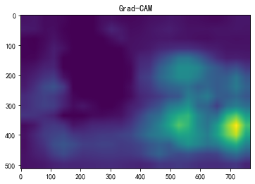
targets = [ClassifierOutputTarget(232)]

cam_map = cam(input_tensor=input_tensor, targets=targets)[0] # 不加平滑

plt.imshow(cam_map)
plt.title('Grad-CAM')
plt.show()

png

import torchcam
from torchcam.utils import overlay_mask

result = overlay_mask(img_pil, Image.fromarray(cam_map), alpha=0.7)
result

在这里插入图片描述

基于Guided Grad-CAM的高分辨率细粒度可解释性分析

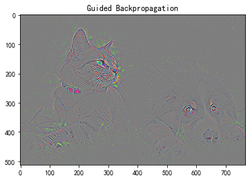
Guided Backpropagation算法

from pytorch_grad_cam import GuidedBackpropReLUModel
from pytorch_grad_cam.utils.image import show_cam_on_image, deprocess_image, preprocess_image

# 初始化算法
gb_model = GuidedBackpropReLUModel(model=model, use_cuda=True)
# 生成 Guided Backpropagation热力图
gb_origin = gb_model(input_tensor, target_category=None)
gb_show = deprocess_image(gb_origin)

plt.imshow(gb_show)
plt.title('Guided Backpropagation')
plt.show()

png

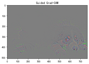
将Grad-CAM热力图与Gudied Backpropagation热力图逐元素相乘

# Grad-CAM三通道热力图
cam_mask = cv2.merge([cam_map, cam_map, cam_map])

# 逐元素相乘
guided_gradcam = deprocess_image(cam_mask * gb_origin)

plt.imshow(guided_gradcam)
plt.title('Guided Grad-CAM')
plt.show()

png

Captum的工具包

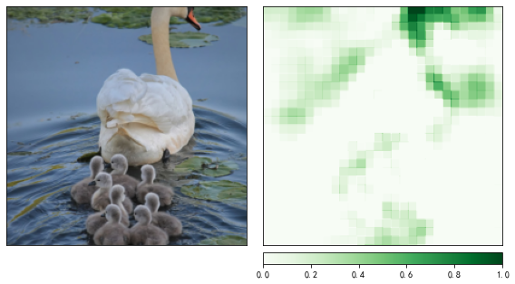
遮挡可解释性分析

这里介绍一部分Captum的方法，也就是遮挡可解释性分析-ImageNet图像分类

在输入图像上，用遮挡滑块，滑动遮挡不同区域，探索哪些区域被遮挡后会显著影响模型的分类决策。

提示：因为每次遮挡都需要分别单独预测，因此代码运行可能需要较长时间。

model = models.resnet18(weights=models.ResNet18_Weights.DEFAULT)
model = model.eval().to(device)

occlusion = Occlusion(model)

中等遮挡滑块

# 获得输入图像每个像素的 occ 值
attributions_occ = occlusion.attribute(input_tensor,
                                       strides = (3, 8, 8), # 遮挡滑动移动步长
                                       target=pred_id, # 目标类别
                                       sliding_window_shapes=(3, 15, 15), # 遮挡滑块尺寸
                                       baselines=0) # 被遮挡滑块覆盖的像素值

# 转为 224 x 224 x 3的数据维度
attributions_occ_norm = np.transpose(attributions_occ.detach().cpu().squeeze().numpy(), (1,2,0))

viz.visualize_image_attr_multiple(attributions_occ_norm, # 224 224 3
                                  rc_img_norm,           # 224 224 3
                                  ["original_image", "heat_map"],
                                  ["all", "positive"],
                                  show_colorbar=True,
                                  outlier_perc=2)
plt.show()

png

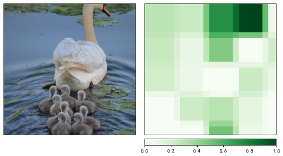
大遮挡滑块

# 更改遮挡滑块的尺寸
attributions_occ = occlusion.attribute(input_tensor,
                                       strides = (3, 50, 50), # 遮挡滑动移动步长
                                       target=pred_id, # 目标类别
                                       sliding_window_shapes=(3, 60, 60), # 遮挡滑块尺寸
                                       baselines=0)

# 转为 224 x 224 x 3的数据维度
attributions_occ_norm = np.transpose(attributions_occ.detach().cpu().squeeze().numpy(), (1,2,0))

viz.visualize_image_attr_multiple(attributions_occ_norm, # 224 224 3
                                  rc_img_norm,           # 224 224 3
                                  ["original_image", "heat_map"],
                                  ["all", "positive"],
                                  show_colorbar=True,
                                  outlier_perc=2)
plt.show()

png

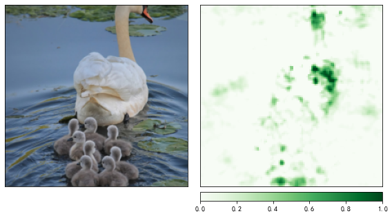
小遮挡滑块

# 更改遮挡滑块的尺寸
attributions_occ = occlusion.attribute(input_tensor,
                                       strides = (3, 2, 2), # 遮挡滑动移动步长
                                       target=pred_id, # 目标类别
                                       sliding_window_shapes=(3, 4, 4), # 遮挡滑块尺寸
                                       baselines=0)

# 转为 224 x 224 x 3的数据维度
attributions_occ_norm = np.transpose(attributions_occ.detach().cpu().squeeze().numpy(), (1,2,0))

viz.visualize_image_attr_multiple(attributions_occ_norm, # 224 224 3
                                  rc_img_norm,           # 224 224 3
                                  ["original_image", "heat_map"],
                                  ["all", "positive"],
                                  show_colorbar=True,
                                  outlier_perc=2)
plt.show()

png

Integrated Gradients可解释性分析

Integrated Gradients原理：输入图像像素由空白变为输入图像像素的过程中，模型预测为某一特定类别的概率相对于输入图像像素的梯度积分。

from captum.attr import IntegratedGradients
from captum.attr import NoiseTunnel

# 初始化可解释性分析方法
integrated_gradients = IntegratedGradients(model)

# 获得输入图像每个像素的 IG 值
attributions_ig = integrated_gradients.attribute(input_tensor, target=pred_id, n_steps=50)
# 转为 224 x 224 x 3的数据维度
attributions_ig_norm = np.transpose(attributions_ig.detach().cpu().squeeze().numpy(), (1,2,0))

from matplotlib.colors import LinearSegmentedColormap

# 设置配色方案
default_cmap = LinearSegmentedColormap.from_list('custom blue', 
                                                 [(0, '#ffffff'),
                                                  (0.25, '#000000'),
                                                  (1, '#000000')], N=256)

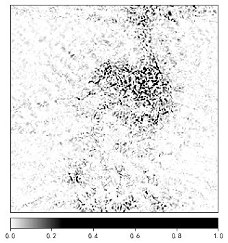
# 可视化 IG 值
viz.visualize_image_attr(attributions_ig_norm, # 224,224,3
                         rc_img_norm,          # 224,224,3
                         method='heat_map',
                         cmap=default_cmap,
                         show_colorbar=True,
                         sign='positive',
                         outlier_perc=1)
plt.show()

png

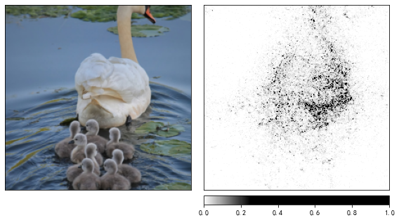
加入高斯噪声的多张图像，平滑输出

在输入图像中加入高斯噪声，构造nt_samples个噪声样本，分别计算IG值，再使用smoothgrad_sq（先平均再平方）平滑。

noise_tunnel = NoiseTunnel(integrated_gradients)

# 获得输入图像每个像素的 IG 值
attributions_ig_nt = noise_tunnel.attribute(input_tensor, nt_samples=3, nt_type='smoothgrad_sq', target=pred_id)

# 转为 224 x 224 x 3的数据维度
attributions_ig_nt_norm = np.transpose(attributions_ig_nt.squeeze().cpu().detach().numpy(), (1,2,0))

# 设置配色方案
default_cmap = LinearSegmentedColormap.from_list('custom blue', 
                                                 [(0, '#ffffff'),
                                                  (0.25, '#000000'),
                                                  (1, '#000000')], N=256)

viz.visualize_image_attr_multiple(attributions_ig_nt_norm, # 224 224 3
                                  rc_img_norm, # 224 224 3
                                  ["original_image", "heat_map"],
                                  ["all", "positive"],
                                  cmap=default_cmap,
                                  show_colorbar=True)
plt.show()

png

总结

在这次任务中，主要学习到了CAM和Captum工具包的使用，在图像分类的基础上去解释他，知其然还要知其所以然。使用CAM和Captum工具包，可以减少我们很多很多的代码量，并且能快速使用，快速应用在自己的任务中、

在经过一个多星期的学习，也是需要这种代码实战告诉我们，这些应用是全面且方方面面的，这样就不会空读理论，这样可以让我们有机会将理论和实践结合起来，希望后续能够将XAI和CAM运用到我的领域中，学习到更多的知识。

参考阅读

可以根据按照代码教程:https://github.com/TommyZihao/Train_Custom_Dataset，用pytorch训练自己的图像分类模型，基于torch-cam实现各个类别、单张图像、视频文件、摄像头实时画面的CAM可视化
Grad-CAM官方代码:https://github.com/ramprs/grad-cam
torch-cam代码库:https://github.com/frgfm/torch-cam
pytorch-grad-cam代码库:https://github.com/jacobgil/pytorch-grad-cam

【学习打卡05】可解释机器学习笔记之CAM+Captum代码实战