活动地址：CSDN21天学习挑战赛

项目数据及源码

可在github下载：

https://github.com/chenshunpeng/Pytorch-framework-predicts-temperature

在这里插入图片描述

数据集1（含friend数据项）

数据预处理

引入库文件：

import numpy as np
import pandas as pd
import matplotlib.pyplot as plt
import torch
import torch.optim as optim
import warnings

warnings.filterwarnings("ignore")
%matplotlib inline

# 加入下述代码！可能！是因为torch包中包含了名为libiomp5md.dll的文件，
# 与Anaconda环境中的同一个文件出现了某种冲突，所以需要删除一个。
import os
os.environ["KMP_DUPLICATE_LIB_OK"]="TRUE"

读入数据：

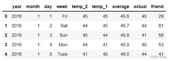
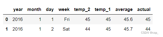
features = pd.read_csv('data1.csv')

# 查看数据（默认查看前5行）
# https://blog.csdn.net/qq_40305043/article/details/104851766
features.head()

结果：
在这里插入图片描述
处理时间数据：

# 处理时间数据
import datetime

# 分别得到年，月，日
years = features['year']
months = features['month']
days = features['day']

# datetime格式
dates = [
    str(int(year)) + '-' + str(int(month)) + '-' + str(int(day))
    for year, month, day in zip(years, months, days)
]

# datetime模块的datetime对象提供的strptime方法可以将字符串转为datetime对象，转换时要求字符串内容符合指定的格式。
dates = [datetime.datetime.strptime(date, '%Y-%m-%d') for date in dates]

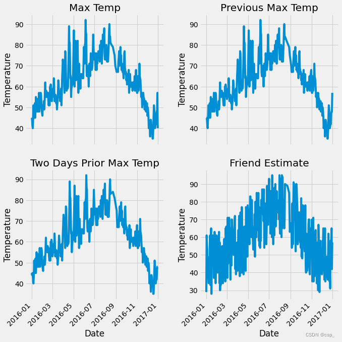
绘制数据图

# 准备画图
# 指定默认风格
plt.style.use('fivethirtyeight')

# 设置布局
fig, ((ax1, ax2), (ax3, ax4)) = plt.subplots(nrows=2,
                                             ncols=2,
                                             figsize=(10, 10))
fig.autofmt_xdate(rotation=45)

# 标签值
ax1.plot(dates, features['actual']) # 所用数据列
ax1.set_xlabel('') # x轴数据
ax1.set_ylabel('Temperature') # y轴数据
ax1.set_title('Max Temp') # 图表标题

# 昨天
ax2.plot(dates, features['temp_1'])
ax2.set_xlabel('')
ax2.set_ylabel('Temperature')
ax2.set_title('Previous Max Temp')

# 前天
ax3.plot(dates, features['temp_2'])
ax3.set_xlabel('Date')
ax3.set_ylabel('Temperature')
ax3.set_title('Two Days Prior Max Temp')

# 朋友预测值（意义不大）
ax4.plot(dates, features['friend'])
ax4.set_xlabel('Date')
ax4.set_ylabel('Temperature')
ax4.set_title('Friend Estimate')

plt.tight_layout(pad=2)

结果：
在这里插入图片描述
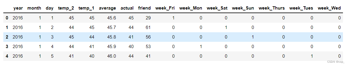
字符串数据转为数值形式：

# 独热编码（字符串数据转为数值形式）
features = pd.get_dummies(features)
features.head(5)

结果：
在这里插入图片描述
在特征中去掉标签actual，把列表转化为数组：

# 标签
labels = np.array(features['actual'])

# 在特征中去掉标签
# axis = 1 表示沿着每一行或者列标签横向执行对应的方法
# https://blog.csdn.net/wyf2017/article/details/107459509
features = features.drop('actual', axis=1)

# 每列的名字单独保存一下，以备后患
feature_list = list(features.columns)

# 转换成合适的格式
# np.array()把列表转化为数组
features = np.array(features)

网络模型结构图

构建2层神经网络（只有1个隐含层），第1层有128个神经元，第2层有1个神经元，其结构可理解为：

[348,14]->[14,128]->[128,1]（输入层->隐含层->输出层）

在这里插入图片描述

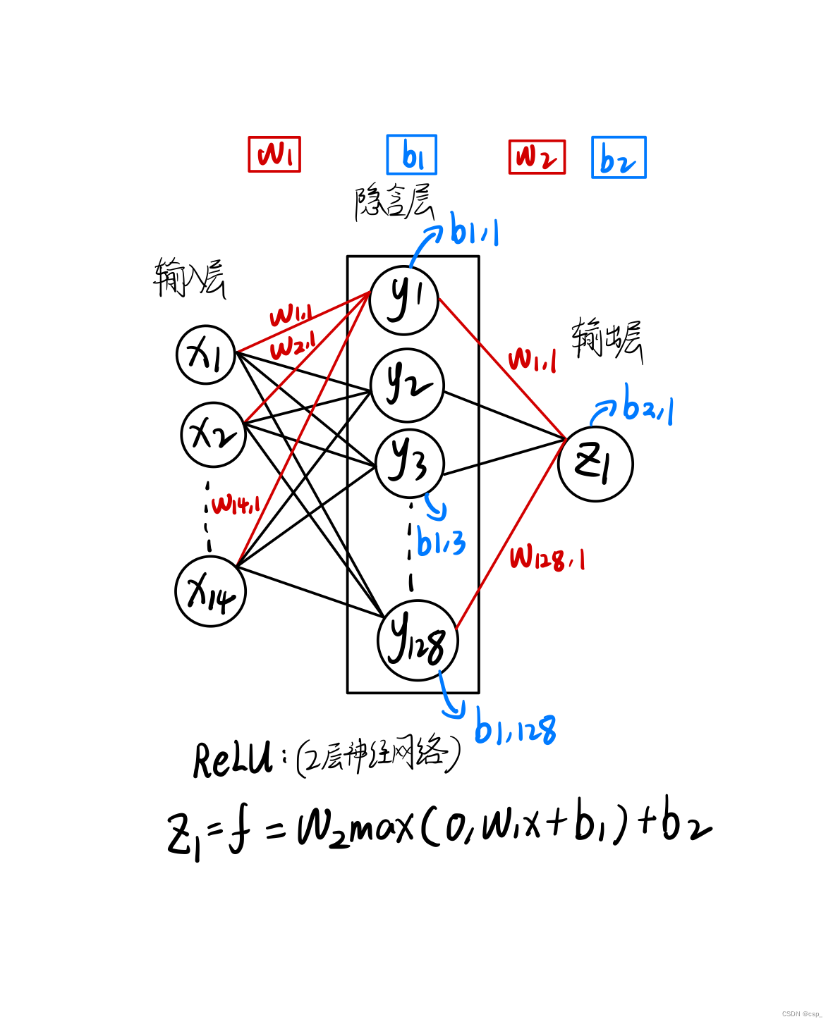
①手动构建网络模型（CPU训练）

weights表示随机生成输入层至隐藏层权重，biases表示随机生成输入层至隐藏层偏移
由于只有单隐藏层，故 weights2 表示隐藏层至输出层权重，biases2 表示隐藏层至输出层的偏移
反向传播计算，反向传播是将当前求出的损失率进行由输出层至输入层的一个方向求偏导的过程，反向求导旨在优化参数w，使得误差更小
在反向传播完成后，计算梯度，并进行w1，w2，b1，b2的更新，更新操作为，沿着梯度的反方向进行学习率*梯度的更新，在每次更新完毕后迭代清空

x = torch.tensor(input_features, dtype=float)

y = torch.tensor(labels, dtype=float)

# 权重参数初始化，构建2层神经网络 （只有1个隐含层）
# [348,14]->[14,128]->[128,1]（输入层->隐含层->输出层）
# 第1层有128个神经元
# randn，从标准正态分布中返回⼀个或多个样本值
weights = torch.randn((14, 128), dtype=float, requires_grad=True) #权值矩阵w
biases = torch.randn(128, dtype=float, requires_grad=True) # 偏置向量b
# 第2层有1个神经元
weights2 = torch.randn((128, 1), dtype=float, requires_grad=True)
biases2 = torch.randn(1, dtype=float, requires_grad=True)

learning_rate = 0.001
losses = []

for i in range(1000):
    # 计算隐层
    hidden = x.mm(weights) + biases
    # 加入激活函数
    hidden = torch.relu(hidden)
    # 预测结果
    predictions = hidden.mm(weights2) + biases2
    # 通计算损失
    loss = torch.mean((predictions - y)**2)
    losses.append(loss.data.numpy())

    # 打印损失值
    if i % 100 == 0:
        print('loss:', loss)
    #返向传播计算
    loss.backward()

    #更新参数
    weights.data.add_(-learning_rate * weights.grad.data)
    biases.data.add_(-learning_rate * biases.grad.data)
    weights2.data.add_(-learning_rate * weights2.grad.data)
    biases2.data.add_(-learning_rate * biases2.grad.data)

    # 每次迭代都得记得清空
    weights.grad.data.zero_()
    biases.grad.data.zero_()
    weights2.grad.data.zero_()
    biases2.grad.data.zero_()

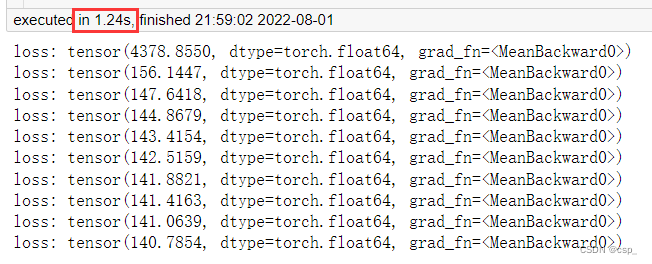
结果：
在这里插入图片描述

②简洁构建网络模型（CPU训练）

初始化网络：

input_size = input_features.shape[1] #样本个数
hidden_size = 128 # 隐含层神经元个数
output_size = 1
batch_size = 16
my_nn = torch.nn.Sequential(
    torch.nn.Linear(input_size, hidden_size), #全连接层
    torch.nn.Sigmoid(), #激活函数
    torch.nn.Linear(hidden_size, output_size),
)
# MSE损失函数
cost = torch.nn.MSELoss(reduction='mean')

# Adam优化器
optimizer = torch.optim.Adam(my_nn.parameters(), lr=0.001)

训练网络：

# 训练网络
losses = []
for i in range(1000):
    batch_loss = []
    # MINI-Batch方法来进行训练
    for start in range(0, len(input_features), batch_size):
        end = start + batch_size if start + batch_size < len(
            input_features) else len(input_features)
        xx = torch.tensor(input_features[start:end],
                          dtype=torch.float,
                          requires_grad=True)
        yy = torch.tensor(labels[start:end],
                          dtype=torch.float,
                          requires_grad=True)
        prediction = my_nn(xx)# 前向传播
        loss = cost(prediction, yy) # 计算损失
        optimizer.zero_grad() # 梯度清零
        loss.backward(retain_graph=True) #反向传播
        optimizer.step() # 更新参数
        batch_loss.append(loss.data.numpy()) #记录损失，便于打印

    # 打印损失
    if i % 100 == 0:
        losses.append(np.mean(batch_loss))
        print(i, np.mean(batch_loss))

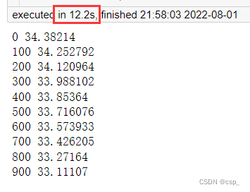
结果：

在这里插入图片描述

预测训练结果

x = torch.tensor(input_features, dtype=torch.float)

# 转换成numpy格式便于画图
predict = my_nn(x).data.numpy()

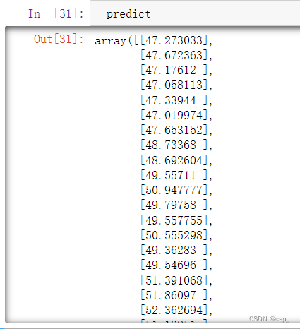
结果：

在这里插入图片描述

在整个过程中，可以对训练过程进行优化的参数有：

损失率
激活函数（大多情况下用relu）
损失的计算，可将方差改为其他损失类型

matplotlib结果可视化

数据设置

# 转换日期格式
dates = [
    str(int(year)) + '-' + str(int(month)) + '-' + str(int(day))
    for year, month, day in zip(years, months, days)
]
dates = [datetime.datetime.strptime(date, '%Y-%m-%d') for date in dates]

# 创建一个表格来存日期和其对应的标签数值
true_data = pd.DataFrame(data={
    
    'date': dates, 'actual': labels})

# 同理，再创建一个来存日期和其对应的模型预测值
months = features[:, feature_list.index('month')]
days = features[:, feature_list.index('day')]
years = features[:, feature_list.index('year')]

test_dates = [
    str(int(year)) + '-' + str(int(month)) + '-' + str(int(day))
    for year, month, day in zip(years, months, days)
]

test_dates = [
    datetime.datetime.strptime(date, '%Y-%m-%d') for date in test_dates
]

predictions_data = pd.DataFrame(data={
    
    
    'date': test_dates,
    'prediction': predict.reshape(-1)
})

绘制图形：

plt.figure(figsize=(20,5))

# 真实值
plt.plot(true_data['date'], true_data['actual'], 'b-', label='actual')

# 预测值
plt.plot(predictions_data['date'],
         predictions_data['prediction'],
         'ro',
         label='prediction')
plt.xticks(rotation='60')
plt.legend()

# 图名
plt.xlabel('Date')
plt.ylabel('Maximum Temperature (F)')
plt.title('Actual and Predicted Values')

结果：

在这里插入图片描述

运行注意

开始运行的时候报错：

在这里插入图片描述

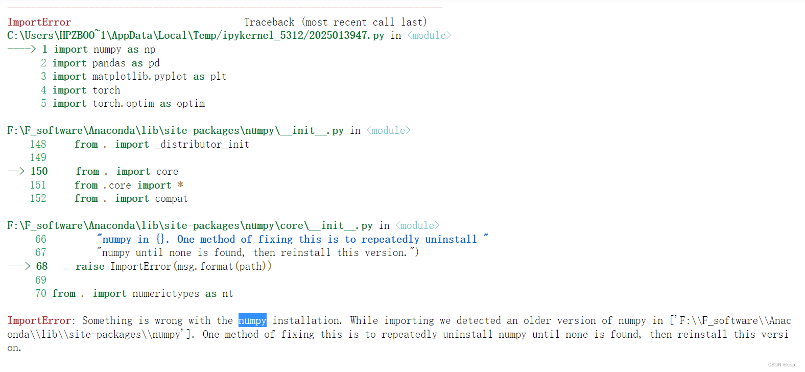
后来发现是安装了2个numpy，这两个numpy版本冲突，首先2次（可能更多）pip uninstall numpy进行卸载

之后pip3 install numpy -i http://pypi.douban.com/simple --trusted-host pypi.douban.com 安装numpy即可

之后给出警告：

在这里插入图片描述

发现：“numexpr”的版本需要更新，至少为2.7.0，输入命令pip install --user numexpr==2.7.0 -i http://pypi.douban.com/simple --trusted-host pypi.douban.com更新即可

数据集2（不含friend数据项）

数据清洗

# 用pandas中的read_csv()函数读取出data1.csv文件中的数据:

import pandas as pd

df = pd.read_csv("data1.csv")
df.head(2)

# 要删除的列的名称为 "friend" 
# 删除指定列
# 参数axis=0，表示对行进行操作，如对列进行操作则更改默认参数为axis=1。

df=df.drop(['friend'],axis=1)

# 保存新的csv文件为data2.csv：
# 参数index=False，表示输出不显示index(索引)值。
# 参数encoding=“utf-8”，表示保存的文件编码格式为utf-8。

df.to_csv("data2.csv",index=False,encoding="utf-8")

读入数据：

df = pd.read_csv("data2.csv")
df.head(2)

结果：
在这里插入图片描述

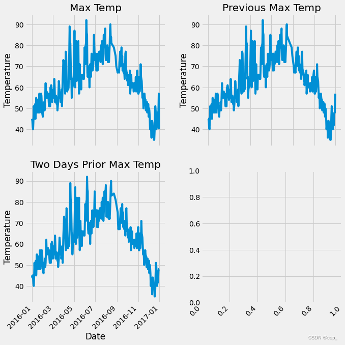
绘制数据图

import numpy as np
import pandas as pd
import matplotlib.pyplot as plt
import torch
import torch.optim as optim
import warnings

warnings.filterwarnings("ignore")
%matplotlib inline

# 加入下述代码！可能！是因为torch包中包含了名为libiomp5md.dll的文件，
# 与Anaconda环境中的同一个文件出现了某种冲突，所以需要删除一个。
import os
os.environ["KMP_DUPLICATE_LIB_OK"]="TRUE"

features = pd.read_csv('data2.csv')

# 处理时间数据
import datetime

# 分别得到年，月，日
years = features['year']
months = features['month']
days = features['day']

# datetime格式
dates = [
    str(int(year)) + '-' + str(int(month)) + '-' + str(int(day))
    for year, month, day in zip(years, months, days)
]

# datetime模块的datetime对象提供的strptime方法可以将字符串转为datetime对象，转换时要求字符串内容符合指定的格式。
dates = [datetime.datetime.strptime(date, '%Y-%m-%d') for date in dates]

# 准备画图
# 指定默认风格
plt.style.use('fivethirtyeight')

# 设置布局
fig, ((ax1, ax2), (ax3, ax4)) = plt.subplots(nrows=2,
                                             ncols=2,
                                             figsize=(10, 10))
fig.autofmt_xdate(rotation=45)

# 标签值
ax1.plot(dates, features['actual']) # 所用数据列
ax1.set_xlabel('') # x轴数据
ax1.set_ylabel('Temperature') # y轴数据
ax1.set_title('Max Temp') # 图表标题

# 昨天
ax2.plot(dates, features['temp_1'])
ax2.set_xlabel('')
ax2.set_ylabel('Temperature')
ax2.set_title('Previous Max Temp')

# 前天
ax3.plot(dates, features['temp_2'])
ax3.set_xlabel('Date')
ax3.set_ylabel('Temperature')
ax3.set_title('Two Days Prior Max Temp')


plt.tight_layout(pad=2)

结果：

在这里插入图片描述
数据处理

# 独热编码（字符串数据转为数值形式）
features = pd.get_dummies(features)

# 标签
labels = np.array(features['actual'])

# 在特征中去掉标签
# axis = 1 表示沿着每一行或者列标签横向执行对应的方法
# https://blog.csdn.net/wyf2017/article/details/107459509
features = features.drop('actual', axis=1)

# 每列的名字单独保存一下，以备后患
feature_list = list(features.columns)

# 转换成合适的格式
# np.array()把列表转化为数组
features = np.array(features)

from sklearn import preprocessing

# 不仅计算训练数据的均值和方差，还会基于计算出来的均值和方差来转换训练数据，从而把数据转换成标准的正太分布
input_features = preprocessing.StandardScaler().fit_transform(features)

构建网络模型（GPU训练）

代码报错的解决方案：

训练神经网络时报错：can’t convert cuda:0 device type tensor to numpy. Use Tensor.cpu() to copy the tensor to host memory first.

正确代码：

input_size = input_features.shape[1]  #样本个数
hidden_size = 128  # 隐含层神经元个数
output_size = 1
batch_size = 16
my_nn = torch.nn.Sequential(
    torch.nn.Linear(input_size, hidden_size),  #全连接层
    torch.nn.Sigmoid(),  #激活函数
    torch.nn.Linear(hidden_size, output_size),
)
# MSE损失函数
cost = torch.nn.MSELoss(reduction='mean')

# Adam优化器
optimizer = torch.optim.Adam(my_nn.parameters(), lr=0.001)

device = torch.device("cuda:0" if torch.cuda.is_available() else "cpu")
print(device)

my_nn.to(device)

# 训练网络
losses = []
for i in range(1000):
    batch_loss = []
    # MINI-Batch方法来进行训练
    for start in range(0, len(input_features), batch_size):
        
        input_features.to(device)
        labels.to(device)
        
        end = start + batch_size if start + batch_size < len(
            input_features) else len(input_features)
        xx = torch.tensor(input_features[start:end],
                          dtype=torch.float,
                          requires_grad=True)
        yy = torch.tensor(labels[start:end],
                          dtype=torch.float,
                          requires_grad=True)

        prediction = my_nn(xx)  # 前向传播
        loss = cost(prediction, yy)  # 计算损失
        optimizer.zero_grad()  # 梯度清零
        loss.backward(retain_graph=True)  #反向传播
        optimizer.step()  # 更新参数
#         batch_loss.append(loss.data.numpy())  #记录损失，便于打印
        batch_loss.append(loss.data.cpu().numpy())  #记录损失，便于打印


    # 打印损失
    if i % 100 == 0:
        losses.append(np.mean(batch_loss))
        print(i, np.mean(batch_loss))

结果：

在这里插入图片描述

matplotlib结果可视化

x = torch.tensor(input_features, dtype=torch.float)

# 转换成numpy格式便于画图
predict = my_nn(x).data.numpy()

# 转换日期格式
dates = [
    str(int(year)) + '-' + str(int(month)) + '-' + str(int(day))
    for year, month, day in zip(years, months, days)
]
dates = [datetime.datetime.strptime(date, '%Y-%m-%d') for date in dates]

# 创建一个表格来存日期和其对应的标签数值
true_data = pd.DataFrame(data={
    
    'date': dates, 'actual': labels})

# 同理，再创建一个来存日期和其对应的模型预测值
months = features[:, feature_list.index('month')]
days = features[:, feature_list.index('day')]
years = features[:, feature_list.index('year')]

test_dates = [
    str(int(year)) + '-' + str(int(month)) + '-' + str(int(day))
    for year, month, day in zip(years, months, days)
]

test_dates = [
    datetime.datetime.strptime(date, '%Y-%m-%d') for date in test_dates
]

predictions_data = pd.DataFrame(data={
    
    
    'date': test_dates,
    'prediction': predict.reshape(-1)
})

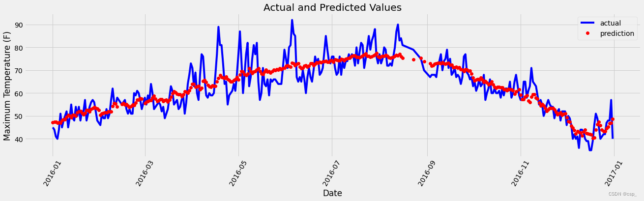
plt.figure(figsize=(20,5))

# 真实值
plt.plot(true_data['date'], true_data['actual'], 'b-', label='actual')

# 预测值
plt.plot(predictions_data['date'],
         predictions_data['prediction'],
         'ro',
         label='prediction')
plt.xticks(rotation='60')
plt.legend()

# 图名
plt.xlabel('Date')
plt.ylabel('Maximum Temperature (F)')
plt.title('Actual and Predicted Values')

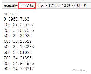
训练结果：

0 3870.6526
100 37.636475
200 35.619022
300 35.33533
400 35.18585
500 35.07154
600 34.970573
700 34.8705
800 34.767883
900 34.66196

可视化：

在这里插入图片描述

结论

数据集的优化对结果影响不大，因此改进网络结构才是优化的关键所在

网络结构比较小的时候，CPU与GPU数据传输过程耗时更高，这个时候只用CPU会更快

网络结构比较庞大的时候，GPU的提速就比较明显了

PyTorch构建神经网络预测气温（数据集对比，CPU与GPU对比）

目录

项目数据及源码

数据集1（含friend数据项）

数据预处理

绘制数据图

网络模型结构图

①手动构建网络模型（CPU训练）

②简洁构建网络模型（CPU训练）

matplotlib结果可视化

运行注意

数据集2（不含friend数据项）

数据清洗

绘制数据图

构建网络模型（GPU训练）

matplotlib结果可视化

结论

猜你喜欢