【PyTorch量化实践（2）】

---

翻译来源https://pytorch.org/blog/quantization-in-practice/

量化是一种廉价而简单的方法，可以使深度神经网络模型运行得更快，并具有更低的内存需求。PyTorch提供了几种量化模型的不同方法。在这篇博客文章中，我们将(快速)为深度学习中的量化奠定基础，然后看看每种技术在实践中是怎样的。最后，我们将以文献中关于在工作流程中使用量化的建议作为结束。

量化方法

PyTorch允许使用几种不同的方法来量化模型：

• 如果更喜欢灵活但手动的，或有限制的自动过程（Eager模式和FX Graph模式）
• 如果量化激活(层输出)的qparams为所有输入预先进行计算，或者对每个输入重新计算（静态和动态）
• 计算qparams后是否进行了再训练（quantization-aware training 和 post-training
  quantization）

FX Graph模式自动融合符合条件的模块，插入Quant/DeQuant stubs，校准模型并返回一个量化模块，所有这些都在两个方法调用中，但只适用于符号可跟踪（symbolic traceable）的网络。后面的示例包含使用Eager Mode和FX Graph Mode进行比较的调用

在DNNs中，有资格进行量化的候选是FP32权重(layer参数)和激活(layer输出)。量化权重可以减小模型尺寸。量化的激活通常会导致更快的推断。例如，50层的ResNet网络有~ 2600万个权重参数，在前向传递中计算~ 1600万个激活。

Post-Training Dynamic/Weight-only Quantization预训练后动态量化

这里模型的权重是预先量化的。在推理过程中，激活被实时量化(“动态”)。这是所有方法中最简单的一种，它在torch. quantized .quantize_dynamic中只有一行API调用。目前只支持线性和递归(LSTM, GRU, RNN)层进行动态量化。

优点：

• 可产生更高的精度，因为剪切范围精确校准每个输入
• 对于LSTMs和transformer这样的模型，动态量化是首选，在这些模型中，从内存中写入/检索模型的权重占主导带宽

缺点：

• 在运行时对每一层的激活进行校准和量化会增加计算开销。

import torch
from torch import nn

# toy model
m = nn.Sequential(
  nn.Conv2d(2, 64, (8,)),
  nn.ReLU(),
  nn.Linear(16,10),
  nn.LSTM(10, 10))

m.eval()

## EAGER MODE
from torch.quantization import quantize_dynamic
model_quantized = quantize_dynamic(
    model=m, qconfig_spec={
    
    nn.LSTM, nn.Linear}, dtype=torch.qint8, inplace=False
)

## FX MODE
from torch.quantization import quantize_fx
qconfig_dict = {
    
    "": torch.quantization.default_dynamic_qconfig}  # An empty key denotes the default applied to all modules
model_prepared = quantize_fx.prepare_fx(m, qconfig_dict)
model_quantized = quantize_fx.convert_fx(model_prepared)

Post-Training Static Quantization (PTQ)预训练后静态量化

PTQ也是预量化模型权重，但不是实时校准激活，而是使用验证数据预校准和固定(“静态”)的剪切范围。在推理期间，操作之间的激活保持量化的精度。大约100个小批次的代表性数据足以校准观察者的[2]。为了方便起见，下面的例子在校准时使用了随机数据——在应用程序中使用它将导致错误的qparams。

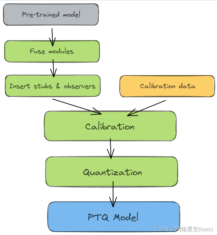
模块融合将多个顺序模块(如:[Conv2d, BatchNorm, ReLU])合并为一个模块。融合模块意味着编译器只需要运行一个内核，而不是多个；这可以通过减少量化误差来加快速度和提高准确性。

优点：

• 静态量化比动态量化具有更快的推断速度，因为它消除了层之间的float<->int转换开销。

缺点：

• 静态量化模型可能需要定期重新校准，以保持对分布漂移的鲁棒性。

# Static quantization of a model consists of the following steps:

#     Fuse modules
#     Insert Quant/DeQuant Stubs
#     Prepare the fused module (insert observers before and after layers)
#     Calibrate the prepared module (pass it representative data)
#     Convert the calibrated module (replace with quantized version)

import torch
from torch import nn

backend = "fbgemm"  # running on a x86 CPU. Use "qnnpack" if running on ARM.

m = nn.Sequential(
    nn.Conv2d(2, 64, 3),
    nn.ReLU(),
    nn.Conv2d(64, 128, 3),
    nn.ReLU()
)
## EAGER MODE
"""Fuse
- Inplace fusion replaces the first module in the sequence with the fused module, and the rest with identity modules
"""
torch.quantization.fuse_modules(m, ['0', '1'], inplace=True)  # fuse first Conv-ReLU pair
torch.quantization.fuse_modules(m, ['2', '3'], inplace=True)  # fuse second Conv-ReLU pair

"""Insert stubs"""
m = nn.Sequential(torch.quantization.QuantStub(),
                  *m,
                  torch.quantization.DeQuantStub())

"""Prepare"""
m.qconfig = torch.quantization.get_default_qconfig(backend)
torch.quantization.prepare(m, inplace=True)

"""Calibrate
- This example uses random data for convenience. Use representative (validation) data instead.
"""
with torch.no_grad():
    for _ in range(10):
        x = torch.rand(1, 2, 28, 28)
        m(x)

"""Convert"""
torch.quantization.convert(m, inplace=True)

"""Check"""
print(m[1].weight().element_size())  # 1 byte instead of 4 bytes for FP32

## FX GRAPH
from torch.quantization import quantize_fx

model_to_quantize = nn.Sequential(
    nn.Conv2d(2, 64, 3),
    nn.ReLU(),
    nn.Conv2d(64, 128, 3),
    nn.ReLU()
)
model_to_quantize.eval()
qconfig_dict = {
    
    "": torch.quantization.get_default_qconfig(backend)}
# Prepare
model_prepared = quantize_fx.prepare_fx(model_to_quantize, qconfig_dict)
# Calibrate - Use representative (validation) data.
with torch.no_grad():
    for _ in range(10):
        x = torch.rand(1, 2, 28, 28)
        model_prepared(x)
# quantize
model_quantized = quantize_fx.convert_fx(model_prepared)
print(model_quantized)

Quantization-aware Training (QAT) 量化后训练

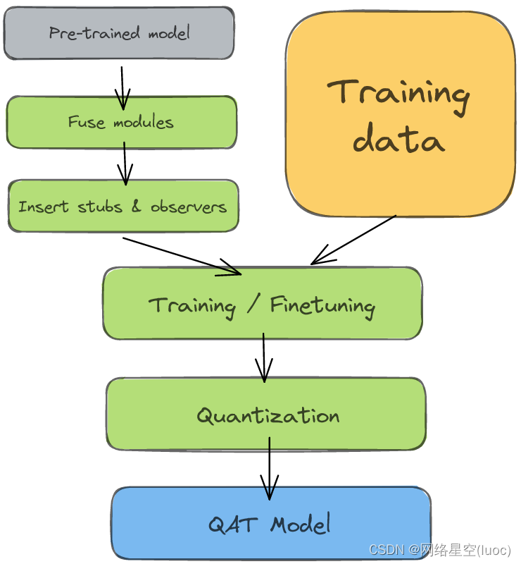
PTQ方法适用于大型模型，但在较小的模型中精度会受到影响。当然，这是由于将FP32的模型调整到INT8领域会造成数值精度的损失(下图a）。QAT通过在训练损失中包含量化误差来解决这一问题，从而训练出一个INT8-first模型。

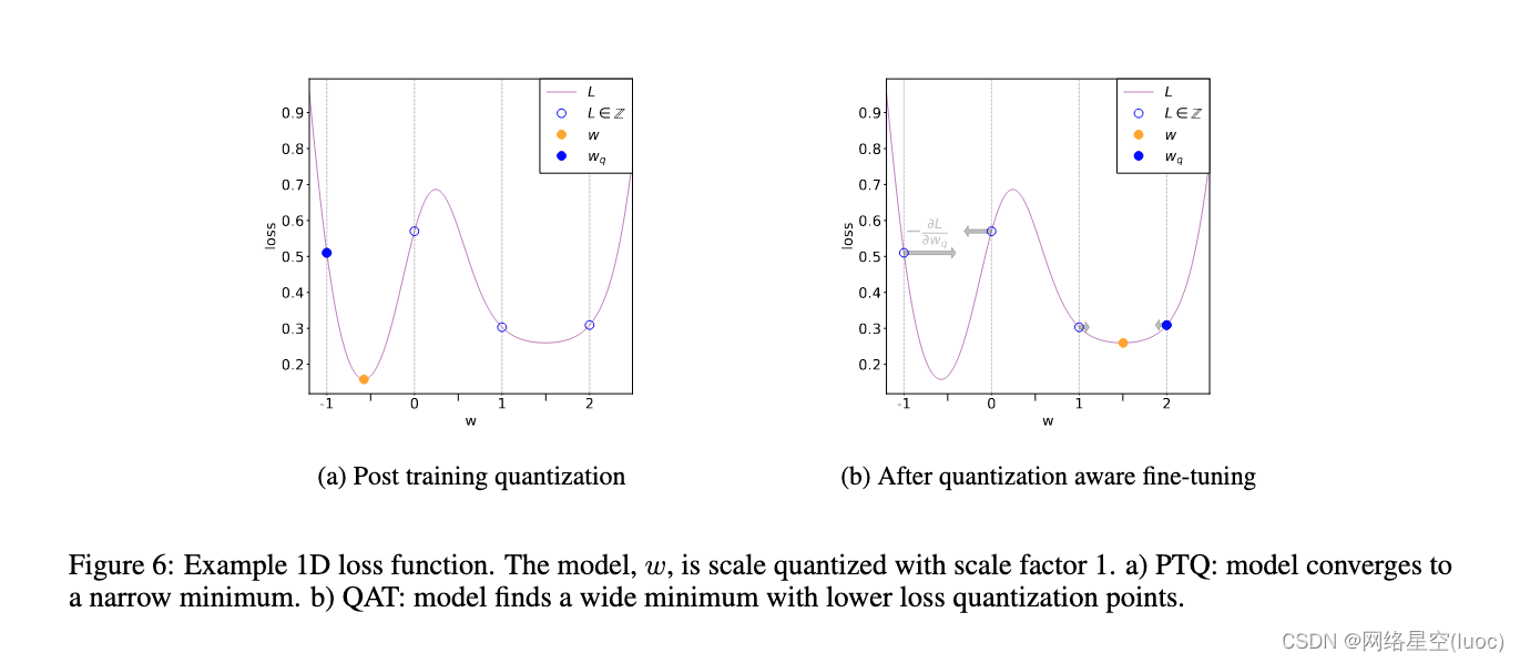
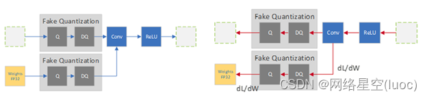
所有的权重和偏差都存储在FP32中，反向传播照常发生。然而，在前向传递中，量化是通过FakeQuantize模块进行内部模拟的。它们之所以被称为假的，是因为它们对数据进行量化并立即去量化，添加了类似于量化推断过程中可能遇到的量化噪声。因此，最终的损失解释了任何预期的量化误差。在此基础上进行优化可以使模型识别出损失函数中更大的区域(上图b)，并识别出FP32参数，从而将其量化到INT8中不会出现显著偏差。

特性

• 优点：QAT的准确度高于PTQ。
• 优点：Qparams可以在模型训练期间学习，以获得更细粒度的准确性(参见LearnableFakeQuantize)
• 缺点：模型在QAT中再训练的计算成本可达几百个epoch

# QAT follows the same steps as PTQ, with the exception of the training loop before you actually convert the model to its quantized version

import torch
from torch import nn

backend = "fbgemm"  # running on a x86 CPU. Use "qnnpack" if running on ARM.

m = nn.Sequential(
     nn.Conv2d(2,64,8),
     nn.ReLU(),
     nn.Conv2d(64, 128, 8),
     nn.ReLU()
)

"""Fuse"""
torch.quantization.fuse_modules(m, ['0','1'], inplace=True) # fuse first Conv-ReLU pair
torch.quantization.fuse_modules(m, ['2','3'], inplace=True) # fuse second Conv-ReLU pair

"""Insert stubs"""
m = nn.Sequential(torch.quantization.QuantStub(),
                  *m,
                  torch.quantization.DeQuantStub())

"""Prepare"""
m.train()
m.qconfig = torch.quantization.get_default_qconfig(backend)
torch.quantization.prepare_qat(m, inplace=True)

"""Training Loop"""
n_epochs = 10
opt = torch.optim.SGD(m.parameters(), lr=0.1)
loss_fn = lambda out, tgt: torch.pow(tgt-out, 2).mean()
for epoch in range(n_epochs):
  x = torch.rand(10,2,24,24)
  out = m(x)
  loss = loss_fn(out, torch.rand_like(out))
  opt.zero_grad()
  loss.backward()
  opt.step()
  print(loss)

"""Convert"""
m.eval()
torch.quantization.convert(m, inplace=True)

灵敏度分析

并不是所有层对量化的反应都是一样的，有些层对精确的下降比其他层更敏感。确定能够最大限度降低精度的最佳层组合非常耗时，因此[3]建议进行一次一次的灵敏度分析，以确定哪些层是最敏感的，并在这些层上保持FP32的精度。在他们的实验中，只跳过2个传输层(在MobileNet v1中总共28个传输层)，就能获得接近fp32的精度。使用FX图形模式，我们可以很容易地创建自定义qconfig:

# ONE-AT-A-TIME SENSITIVITY ANALYSIS 

for quantized_layer, _ in model.named_modules():
  print("Only quantizing layer: ", quantized_layer)

  # The module_name key allows module-specific qconfigs. 
  qconfig_dict = {
    
    "": None, 
  "module_name":[(quantized_layer, torch.quantization.get_default_qconfig(backend))]}

  model_prepared = quantize_fx.prepare_fx(model, qconfig_dict)
  # calibrate
  model_quantized = quantize_fx.convert_fx(model_prepared)
  # evaluate(model)

另一种方法是比较FP32和INT8层的统计数据;常用的度量标准是信噪比(信噪比)和均方误差。这种比较分析也有助于指导进一步的优化。

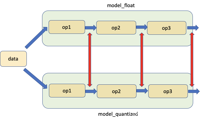
PyTorch在Numeric Suite下提供了帮助进行这种分析的工具。从完整教程了解更多关于使用Numeric Suite的信息。

# extract from https://pytorch.org/tutorials/prototype/numeric_suite_tutorial.html
import torch.quantization._numeric_suite as ns

def SQNR(x, y):
    # Higher is better
    Ps = torch.norm(x)
    Pn = torch.norm(x-y)
    return 20*torch.log10(Ps/Pn)

wt_compare_dict = ns.compare_weights(fp32_model.state_dict(), int8_model.state_dict())
for key in wt_compare_dict:
    print(key, compute_error(wt_compare_dict[key]['float'], wt_compare_dict[key]['quantized'].dequantize()))

act_compare_dict = ns.compare_model_outputs(fp32_model, int8_model, input_data)
for key in act_compare_dict:
    print(key, compute_error(act_compare_dict[key]['float'][0], act_compare_dict[key]['quantized'][0].dequantize()))

量化工作流程建议

要点

• 大(10M+参数)模型对量化误差具有更强的鲁棒性。

• 从FP32检查点量化模型比从零开始训练INT8模型提供了更好的准确性

• 分析模型运行时是可选的，但它可以帮助识别瓶颈推断的层。

• 动态量化是一个简单的第一步，特别是如果你的模型有许多线性或循环层。

• 使用对称的每通道量化与MinMax观察者量化权重。使用带有MovingAverageMinMax观察器的仿射每张量量化激活

• 使用像SQNR这样的指标来识别哪些层最容易出现量化错误。关闭这些层上的量化。

• 使用QAT微调约10%的原始训练计划，退火学习率计划从初始训练学习率的1%开始。