1、pytorch中 torch.nn的介绍
torch.nn是pytorch中自带的一个函数库,里面包含了神经网络中使用的一些常用函数,如具有可学习参数的nn.Conv2d(),nn.Linear()和不具有可学习的参数(如ReLU,pool,DropOut等)(后面这几个是在nn.functional中),这些函数可以放在构造函数中,也可以不放。
通常引入的时候写成:
import torch.nn as nn
import torch.nn.functional as F
这里我们把函数写在了构造函数中:
class ConvNet(nn.Module):
    def __init__(self):
        super().__init__()
        self.conv1 = nn.Conv2d(1, 10, 5) # 输入通道数1,输出通道数10,核的大小5
        self.conv2 = nn.Conv2d(10, 20, 3) # 输入通道数10,输出通道数20,核的大小3
        # 下面的全连接层Linear的第一个参数指输入通道数,第二个参数指输出通道数
        self.fc1 = nn.Linear(20*10*10, 500) # 输入通道数是2000,输出通道数是500
        self.fc2 = nn.Linear(500, 10) # 输入通道数是500,输出通道数是10,即10分类
    def forward(self,x):
        in_size = x.size(0)
        out = self.conv1(x)
        out = F.relu(out)
        out = F.max_pool2d(out, 2, 2)
        out = self.conv2(out)
        out = F.relu(out)
        out = out.view(in_size, -1)
        out = self.fc1(out)
        out = F.relu(out)
        out = self.fc2(out)
        out = F.log_softmax(out, dim=1)
        return out
2、import torch.utils.data
数据加载器,结合了数据集和取样器,并且可以提供多个线程处理数据集。在训练模型时使用到此函数,用来把训练数据分成多个小组,此函数每次抛出一组数据。直至把所有的数据都抛出。就是做一个数据的初始化。
"""
    批训练,把数据变成一小批一小批数据进行训练。
    DataLoader就是用来包装所使用的数据,每次抛出一批数据
"""
import torch
import torch.utils.data as Data

BATCH_SIZE = 5

x = torch.linspace(1, 10, 10) # linspace: 返回一个1维张量,包含在区间start和end上均匀间隔的step个点
y = torch.linspace(10, 1, 10)
# 把数据放在数据集中
torch_dataset = Data.TensorDataset(x, y)
loader = Data.DataLoader(
    # 从数据集中每次抽出batch size个样本
    dataset=torch_dataset,
    batch_size=BATCH_SIZE,
    shuffle=True,
    num_workers=2,
)

def show_batch():
    for epoch in range(3): # epoch: 迭代次数
        print('Epoch:', epoch)
        for batch_id, (batch_x, batch_y) in enumerate(loader):
            print("  batch_id:{}, batch_x:{}, batch_y:{}".format(batch_id, batch_x, batch_y))
            # print(f'  batch_id:{batch_id}, batch_x:{batch_x}, batch_y:{batch_y}')

if __name__ == '__main__':
    show_batch()
输出:
Epoch: 0
  batch_id:0, batch_x:tensor([ 7.,  4.,  3.,  9., 10.]), batch_y:tensor([4., 7., 8., 2., 1.])
  batch_id:1, batch_x:tensor([6., 2., 1., 5., 8.]), batch_y:tensor([ 5.,  9., 10.,  6.,  3.])
Epoch: 1
  batch_id:0, batch_x:tensor([ 2.,  7., 10.,  8.,  3.]), batch_y:tensor([9., 4., 1., 3., 8.])
  batch_id:1, batch_x:tensor([6., 9., 1., 4., 5.]), batch_y:tensor([ 5.,  2., 10.,  7.,  6.])
Epoch: 2
  batch_id:0, batch_x:tensor([10.,  3.,  9.,  6.,  8.]), batch_y:tensor([1., 8., 2., 5., 3.])
  batch_id:1, batch_x:tensor([1., 4., 2., 7., 5.]), batch_y:tensor([10.,  7.,  9.,  4.,  6.])
3、PyTorch中Variable变量与torch.autograd.Variable
顾名思义,Variable就是 变量 的意思。实质上也就是可以变化的量,区别于int变量,它是一种可以变化的变量,这正好就符合了反向传播,参数更新的属性。
具体来说,在pytorch中的Variable就是一个存放会变化值的地理位置,里面的值会不停发生变化,就像一个装鸡蛋的篮子,鸡蛋数会不断发生变化。那谁是里面的鸡蛋呢,自然就是pytorch中的tensor了。(也就是说,pytorch都是有tensor计算的,而tensor里面的参数都是Variable的形式)。如果用Variable计算的话,那返回的也是一个同类型的Variable。
import torch
from torch.autograd import Variable # torch 中 Variable 模块
tensor = torch.FloatTensor([[1,2],[3,4]])
# 把鸡蛋放到篮子里, requires_grad是参不参与误差反向传播, 要不要计算梯度
variable = Variable(tensor, requires_grad=True)

print(tensor)
"""
 1  2
 3  4
[torch.FloatTensor of size 2x2]
"""

print(variable)
"""
Variable containing:
 1  2
 3  4
[torch.FloatTensor of size 2x2]
"""
注:tensor不能反向传播,variable可以反向传播。
Variable求梯度
Variable计算时,它会逐渐地生成计算图。这个图就是将所有的计算节点都连接起来,最后进行误差反向传递的时候,一次性将所有Variable里面的梯度都计算出来,而tensor就没有这个能力。
v_out.backward()    # 模拟 v_out 的误差反向传递

print(variable.grad)    # 初始 Variable 的梯度
'''
 0.5000  1.0000
 1.5000  2.0000
'''
获取Variable里面的数据
直接print(Variable) 只会输出Variable形式的数据,在很多时候是用不了的。所以需要转换一下,将其变成tensor形式。
print(variable)     #  Variable 形式
"""
Variable containing:
 1  2
 3  4
[torch.FloatTensor of size 2x2]
"""

print(variable.data)    # 将variable形式转为tensor 形式
"""
 1  2
 3  4
[torch.FloatTensor of size 2x2]
"""

print(variable.data.numpy())    # numpy 形式
"""
[[ 1.  2.]
 [ 3.  4.]]
"""
4、torch.max()
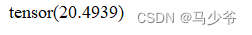
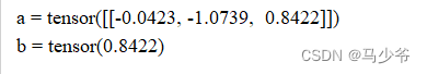
torch.max(input) → Tensor
返回输入tensor中所有元素的最大值
import torch
a = torch.randn(1, 3)
print('a =', a)

b =torch.max(a)
print('b =', b)
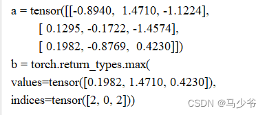
torch.max(input, dim, keepdim=False, out=None) -> (Tensor, LongTensor)
按维度dim 返回最大值
torch.max)(a,0) 返回每一列中最大值的那个元素,且返回索引(返回最大元素在这一列的行索引)
a = torch.randn(3,3)
print('a =', a)

b=torch.max(a,0)
print('b =', b)
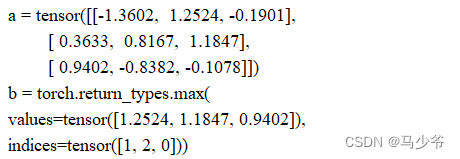
torch.max(a,1) 返回每一行中最大值的那个元素,且返回其索引(返回最大元素在这一行的列索引)
#返回每一行的最大值及索引
a = torch.randn(3,3)
print('a =', a)

b=torch.max(a,1)
print('b =', b)
torch.max()[0], 只返回最大值的每个数
troch.max()[1], 只返回最大值的每个索引
torch.max()[1].data 只返回variable中的数据部分(去掉Variable containing:)
torch.max()[1].data.numpy() 把数据转化成numpy ndarry
torch.max()[1].data.numpy().squeeze() 把数据条目中维度为1 的删除掉
torch.max(tensor1,tensor2) element-wise 比较tensor1 和tensor2 中的元素,返回较大的那个值
5、nn.Linear()
PyTorch的nn.Linear()是用于设置网络中的全连接层的,需要注意在二维图像处理的任务中,全连接层的输入与输出一般都设置为二维张量,形状通常为[batch_size, size],不同于卷积层要求输入输出是四维张量。其用法与形参说明如下
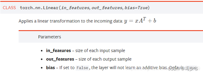
in_features指的是输入的二维张量的大小,即输入的[batch_size, size]中的size。
out_features指的是输出的二维张量的大小,即输出的二维张量的形状为[batch_size,output_size],当然,它也代表了该全连接层的神经元个数。
从输入输出的张量的shape角度来理解,相当于一个输入为[batch_size, in_features]的张量变换成了[batch_size, out_features]的输出张量。
用法示例:
import torch as t
from torch import nn
# in_features由输入张量的形状决定,out_features则决定了输出张量的形状
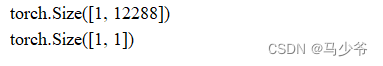
connected_layer = nn.Linear(in_features = 64*64*3, out_features = 1)
# 假定输入的图像形状为[64,64,3]
input = t.randn(1,64,64,3)
# 将四维张量转换为二维张量之后,才能作为全连接层的输入
input = input.view(1,64*64*3)
print(input.shape)
output = connected_layer(input) # 调用全连接层
print(output.shape)
6、torch.bmm()
计算两个tensor的矩阵乘法,torch.bmm(a,b),tensor a 的size为(b,h,w),tensor b的size为(b,w,m) 也就是说两个tensor的第一维是相等的,然后第一个数组的第三维和第二个数组的第二维度要求一样,对于剩下的则不做要求,输出维度 (b,h,m)
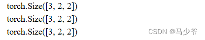
a=torch.Tensor([[[3,4],[1,2]],[[3,4],[1,2]],[[3,4],[1,2]]])
b=torch.Tensor([[[1,2],[3,4]],[[1,2],[3,4]],[[3,4],[1,2]]])
print(a.shape)
print(b.shape)
c = torch.bmm(a,b)
print(c.shape)
7、torch.norm
inputs的一共N维的话对这N个数据求p范数,当然这个还是太抽象了,接下来还是看具体的代码~
p指的是求p范数的p值,函数默认p=2,那么就是求2范数
import torch
rectangle_height = 3
rectangle_width = 4
inputs = torch.randn(rectangle_height, rectangle_width)
for i in range(rectangle_height):
for j in range(rectangle_width):
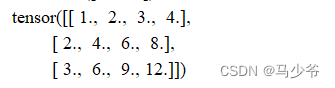
inputs[i][j] = (i + 1) * (j + 1)
print(inputs)
得到一个3×4矩阵,如下
接着我们分别对其行和列分别求2范数
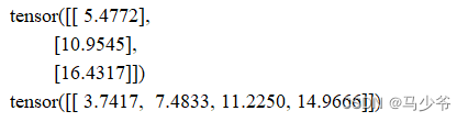
inputs1 = torch.norm(inputs, p=2, dim=1, keepdim=True)
print(inputs1)
inputs2 = torch.norm(inputs, p=2, dim=0, keepdim=True)
print(inputs2)
关注keepdim = False这个参数
inputs3 = inputs.norm(p=2, dim=1, keepdim=False)
print(inputs3)

输出inputs1和inputs3的shape
print(inputs1.shape)
print(inputs3.shape)
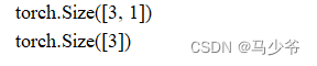
可以看到inputs3少了一维,其实就是dim=1(求范数)那一维(列)少了,因为从4列变成1列,就是3行中求每一行的2范数,就剩1列了,不保持这一维不会对数据产生影响。
或者也可以这么理解,就是数据每个数据有没有用[]扩起来。
keepdim = True,用[]扩起来;
keepdim = False,不用[]括起来~;
不写keepdim,则默认不保留dim的那个维度
inputs4 = torch.norm(inputs, p=2, dim=1)
print(inputs4)

不写dim,则计算Tensor中所有元素的2范数
inputs5 = torch.norm(inputs, p=2)
print(inputs5)