机器学习笔记 - 探索 keras 数据集

1、概述

        数据集对于功能性机器学习模型至关重要。 拥有一个好的可用数据集可能是您的 ML 项目成功或失败的主要因素。特别是当您不熟悉机器学习以及创建模型以进行学习时尤其如此。

        这就是 Keras 深度学习框架包含一组标准数据集的原因。可以帮助用户确认算法或者模型，今天，我们将更详细地了解这些数据集。我们单独探索数据集，详细查看数据，尽可能可视化内容。 此外，我们将尝试找出这些数据集可能对您的学习轨迹有用的一些用例。

2、Keras Datasets

        为了让对机器学习感兴趣的人能够顺利开始，Keras 在框架的上下文中提供了许多数据集。 这意味着您可以开始创建模型而不必担心数据：您只需要少量代码即可加载它。

        理由很简单：收集数据是机器学习项目中最麻烦的地方。通常，数据以 CSV 工作表、传统 SQL 数据库或更糟的形式 - 在 Word 文档或 PDF 文件中可用。 然后，您必须抓取数据、清理数据并将其存储在 Pandas 数据框之类的东西中，然后才能在机器学习模型中使用它。

        但是如果让初学者（一点都不了解机器学习该怎么入手的）进行数据收集和处理或者找到很复杂的数据集也不知道怎么办，这就是为什么 Keras 只需一个调用就可以轻松加载一些数据集：load_data()。

        Keras内置数据集如下：

        图像分类: CIFAR-10, CIFAR-100, MNIST, Fashion-MNIST；

        文本分类: IMDB Movie Reviews, Reuters Newswire topics；

        回归: Boston House Prices；

        官方api地址。

Module: tf.keras.datasets  |  TensorFlow Core v2.9.1https://tensorflow.google.cn/api_docs/python/tf/keras/datasets

3、数据集

（1）CIFAR-10 小图像分类

        CIFAR-10 数据集由 Krizhevsky & Hinton (2009) 引入，可用于图像分类。 它以资助创建它的项目的加拿大高级研究所 (CIFAR) 命名，它包含 10 个类的 60000 个 RGB 图像 - 每类 6000 个。

        CIFAR-10 有这些类的图像（Krizhevsky & Hinton，2009）：

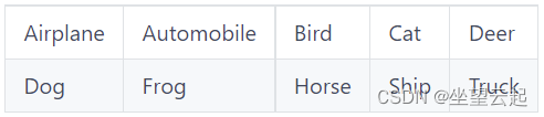
         这些图像是 32 乘以 32 像素，并被分成 50000 张图像的训练集和 10000 张图像的测试集。

        使用 Keras 数据集 API，可以轻松加载它。 在代码中包含数据集如下：

from tensorflow.keras.datasets import cifar10
(x_train, y_train), (x_test, y_test) = cifar10.load_data()

        现在让我们可视化来自 CIFAR-10 数据集的 30 个随机样本，以了解图像内容：

# Imports
import matplotlib.pyplot as plt
import numpy as np
from tensorflow.keras.datasets import cifar10

# CIFAR-10
(x_train, y_train), (x_test, y_test) = cifar10.load_data()

# Target classes: numbers to text
classes = {
  0: 'airplane',
  1: 'automobile',
  2: 'bird',
  3: 'cat',
  4: 'deer',
  5: 'dog',
  6: 'frog',
  7: 'horse',
  8: 'ship',
  9: 'truck'
}

# Visualize 30 random samples
for i in np.random.randint(0, len(x_train)-1, 30):
  # Get data
  sample = x_train[i]
  target = y_train[i][0]
  # Set figure size and axis
  plt.figure(figsize=(1.75, 1.75))
  plt.axis('off')
  # Show data
  plt.imshow(sample)
  plt.title(f'{classes[target]}')
  plt.savefig(f'./{i}.jpg')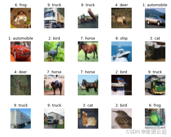

（2）CIFAR-100 小图像分类

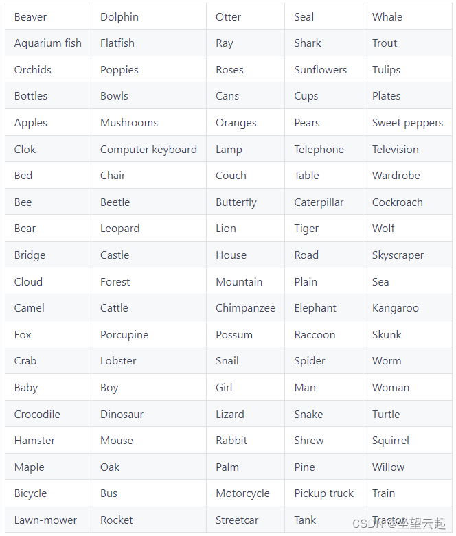
        虽然 CIFAR-10 数据集包含 10 个类的 60000 个样本，但 CIFAR-100 数据集也有 60000 个 - 但这次跨越 100 个非重叠类（Krizhevsky & Hinton，2009）。 CIFAR-100 包含 600 个样本，而不是每个类 6000 个样本。其余部分的结构与 CIFAR-10 数据集非常相似。

from tensorflow.keras.datasets import cifar100
(x_train, y_train), (x_test, y_test) = cifar100.load_data()

        这些是 CIFAR-100 中存在的类（Krizhevsky & Hinton，2009）： 

# Imports
import matplotlib.pyplot as plt
import numpy as np
from tensorflow.keras.datasets import cifar100

# CIFAR-100
(x_train, y_train), (x_test, y_test) = cifar100.load_data()

# Target classes: numbers to text
# Source: https://github.com/keras-team/keras/issues/2653#issuecomment-450133996
classes = [
  'apple',
  'aquarium_fish',
  'baby',
  'bear',
  'beaver',
  'bed',
  'bee',
  'beetle',
  'bicycle',
  'bottle',
  'bowl',
  'boy',
  'bridge',
  'bus',
  'butterfly',
  'camel',
  'can',
  'castle',
  'caterpillar',
  'cattle',
  'chair',
  'chimpanzee',
  'clock',
  'cloud',
  'cockroach',
  'couch',
  'crab',
  'crocodile',
  'cup',
  'dinosaur',
  'dolphin',
  'elephant',
  'flatfish',
  'forest',
  'fox',
  'girl',
  'hamster',
  'house',
  'kangaroo',
  'computer_keyboard',
  'lamp',
  'lawn_mower',
  'leopard',
  'lion',
  'lizard',
  'lobster',
  'man',
  'maple_tree',
  'motorcycle',
  'mountain',
  'mouse',
  'mushroom',
  'oak_tree',
  'orange',
  'orchid',
  'otter',
  'palm_tree',
  'pear',
  'pickup_truck',
  'pine_tree',
  'plain',
  'plate',
  'poppy',
  'porcupine',
  'possum',
  'rabbit',
  'raccoon',
  'ray',
  'road',
  'rocket',
  'rose',
  'sea',
  'seal',
  'shark',
  'shrew',
  'skunk',
  'skyscraper',
  'snail',
  'snake',
  'spider',
  'squirrel',
  'streetcar',
  'sunflower',
  'sweet_pepper',
  'table',
  'tank',
  'telephone',
  'television',
  'tiger',
  'tractor',
  'train',
  'trout',
  'tulip',
  'turtle',
  'wardrobe',
  'whale',
  'willow_tree',
  'wolf',
  'woman',
  'worm',
]

# Visualize 30 random samples
for i in np.random.randint(0, len(x_train)-1, 30):
  # Get data
  sample = x_train[i]
  target = y_train[i][0]
  # Set figure size and axis
  plt.figure(figsize=(1.75, 1.75))
  plt.axis('off')
  # Show data
  plt.imshow(sample)
  plt.title(f'{classes[target]}')
  plt.savefig(f'./{i}.jpg')

（3）IMDB电影评论情感分类

        Maas等人 (2011) 提供用于情感分类的 IMDB 电影评论数据集，该数据集在 Keras 数据集部分进行了预处理。 该数据集包含来自 IMDB 的 25000 条电影评论，按情绪标记（正面和负面）。

        它可用于试验构建情感分类模型。

        如前所述，它是经过预处理的，因此需要描述它是如何进行预处理的。 首先，重要的是要理解“每条评论都被编码为一系列单词索引”。 这意味着每个单词都被转换成一个整数，表示单词在某个单词索引中的位置。 一个样本（准确地说，训练数据中的索引 3）如下所示：

[1, 14, 47, 8, 30, 31, 7, 4, 249, 108, 7, 4, 5974, 54, 61, 369, 13, 71, 149, 14, 22, 112, 4, 2401, 311, 12, 16, 3711, 33, 75, 43, 1829, 296, 4, 86, 320, 35, 534, 19, 263, 4821, 1301, 4, 1873, 33, 89, 78, 12, 66, 16, 4, 360, 7, 4, 58, 316, 334, 11, 4, 1716, 43, 645, 662, 8, 257, 85, 1200, 42, 1228, 2578, 83, 68, 3912, 15, 36, 165, 1539, 278, 36, 69, 44076, 780, 8, 106, 14, 6905, 1338, 18, 6, 22, 12, 215, 28, 610, 40, 6, 87, 326, 23, 2300, 21, 23, 22, 12, 272, 40, 57, 31, 11, 4, 22, 47, 6, 2307, 51, 9, 170, 23, 595, 116, 595, 1352, 13, 191, 79, 638, 89, 51428, 14, 9, 8, 106, 607, 624, 35, 534, 6, 227, 7, 129, 113]

        该值的目标很简单：0。显然，此评论是否定的，尽管我们不知道为什么，因为我们不知道单词:)

        但是，我们可以了解它们。

        我利用了可用于 IMDB 数据集的 get_word_index() 调用的可用性，将 Mdaoust (2019) 创建的一些代码改编为以下代码：

from tensorflow.keras.datasets import imdb
(x_train, y_train), (x_test, y_test) = imdb.load_data()

INDEX_FROM=3   # word index offset
word_to_id = imdb.get_word_index()
word_to_id = {k:(v+INDEX_FROM) for k,v in word_to_id.items()}
word_to_id["<PAD>"] = 0
word_to_id["<START>"] = 1
word_to_id["<UNK>"] = 2
word_to_id["<UNUSED>"] = 3

id_to_word = {value:key for key,value in word_to_id.items()}
print(' '.join(id_to_word[id] for id in x_train[2] ))

        查看内容如下

<START> this has to be one of the worst films of the 1990s when my friends i were watching this film being the target audience it was aimed at we just sat watched the first half an hour with our jaws touching the floor at how bad it really was the rest of the time everyone else in the theatre just started talking to each other leaving or generally crying into their popcorn that they actually paid money they had earnt working to watch this feeble excuse for a film it must have looked like a great idea on paper but on film it looks like no one in the film has a clue what is going on crap acting crap costumes i can't get across how embarrasing this is to watch save yourself an hour a bit of your life

        请注意，实际索引是按词频排序的：i = 1 是最常见的词，i = 2 是第二个最常见的词，依此类推。 这允许例如 “考虑前 10000 个最常用的词，但排除前 20 个 [ones]”。

        在最简单的形式中，可以按如下方式加载数据：

from tensorflow.keras.datasets import imdb
(x_train, y_train), (x_test, y_test) = imdb.load_data()

        但可以设置一些参数：

from tensorflow.keras.datasets import imdb
(x_train, y_train), (x_test, y_test) = imdb.load_data(path="imdb.npz",
                                                      num_words=None,
                                                      skip_top=0,
                                                      maxlen=None,
                                                      seed=113,
                                                      start_char=1,
                                                      oov_char=2,
                                                      index_from=3)

        path：如果您在本地还没有 IMDB 数据，则下载该路径。
        num_words：要考虑的最常见的单词。 超出此值的任何内容都将被编码为 oov_var，正如我们将看到的，它必须由您配置。
        skip_top 告诉 Keras 在开始向 num_words 计数之前要跳过多少个最频繁的单词。
        maxlen 指定序列在被截断之前的最大长度。
        seed是“可重复数据混洗”的随机种子值。 它用于修复打乱数据时使用的随机发生器。
        start_char 向您显示某些序列的开始位置。
        oov_char 替换任何“超出值”的字符（即，因为它超出范围 skip_top < top n word < (num_words + skip_top)）。
        index_from 设置告诉 Keras 数据集从该特定索引中索引单词。

（4）路透社新闻专线主题分类

        另一个文本分类数据集是路透社新闻专线主题数据集。 它的预处理方式与之前的 IMDB 数据集相同，可用于将文本分类为 46 个主题之一：

        来自路透社的 11,228 条新闻专线的数据集，标记了超过 46 个主题。 与 IMDB 数据集一样，每条线路都被编码为一系列单词索引（相同的约定）。

from tensorflow.keras.datasets import reuters
(x_train, y_train), (x_test, y_test) = reuters.load_data()

from tensorflow.keras.datasets import reuters
import numpy as np
(x_train, y_train), (x_test, y_test) = reuters.load_data()

# Define the topics
# Source: https://github.com/keras-team/keras/issues/12072#issuecomment-458154097
topics = ['cocoa','grain','veg-oil','earn','acq','wheat','copper','housing','money-supply',
   'coffee','sugar','trade','reserves','ship','cotton','carcass','crude','nat-gas',
   'cpi','money-fx','interest','gnp','meal-feed','alum','oilseed','gold','tin',
   'strategic-metal','livestock','retail','ipi','iron-steel','rubber','heat','jobs',
   'lei','bop','zinc','orange','pet-chem','dlr','gas','silver','wpi','hog','lead']

# Obtain 3 texts randomly
for i in np.random.randint(0, len(x_train), 3):
  INDEX_FROM=3   # word index offset
  word_to_id = reuters.get_word_index()
  word_to_id = {k:(v+INDEX_FROM) for k,v in word_to_id.items()}
  word_to_id["<PAD>"] = 0
  word_to_id["<START>"] = 1
  word_to_id["<UNK>"] = 2
  word_to_id["<UNUSED>"] = 3

  id_to_word = {value:key for key,value in word_to_id.items()}
  print('=================================================')
  print(f'Sample = {i} | Topic = {topics[y_train[i]]} ({y_train[i]})')
  print('=================================================')
  print(' '.join(id_to_word[id] for id in x_train[i] ))

        在数据集中产生三个文本，关于收入、原油和企业收购，所以看起来：

=================================================
Sample = 8741 | Topic = earn (3)
=================================================
<START> qtly div 50 cts vs 39 cts pay jan 20 record dec 31 reuter 3
=================================================
Sample = 8893 | Topic = crude (16)
=================================================
<START> ice conditions are unchanged at the soviet baltic oil port of ventspils with continuous and compacted drift ice 15 to 30 cms thick the latest report of the finnish board of navigation said icebreaker assistance to reach ventspils harbour is needed for normal steel vessels without special reinforcement against ice the report said it gave no details of ice conditions at the other major soviet baltic export harbour of klaipeda reuter 3
=================================================
Sample = 1829 | Topic = acq (4)
=================================================
<START> halcyon investments a new york firm reported a 6 9 pct stake in research cottrell inc alan slifka a partner in halcyon told reuters the shares were purchased for investment purposes but declined further comment on june 8 research cottrell said it had entered into a definitive agreement to be acquired by r c acquisitions inc for 43 dlrs per share research cottrell closed at 44 1 4 today unchanged from the previous close reuter 3

（5）MNIST 手写数字数据库

        Keras 数据集 API 中包含的另一个数据集是 MNIST 数据集，它代表修改后的国家标准与技术研究所（LeCun 等人）。 该数据集包含 60000 个训练图像和 10000 个手写数字测试图像，它们的大小都是 28 乘以 28 像素。

from tensorflow.keras.datasets import mnist
(x_train, y_train), (x_test, y_test) = mnist.load_data()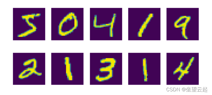

 （6）Fashion-MNIST 时尚文章数据库

        MNIST 数据集在许多研究中用作基准数据集，用于算法验证等。但很多人认为太简单了，不足以有代表性了。Fashion-MNIST数据集是 MNIST 的直接替代品，还包含 60000 个训练图像和 10000 个测试图像。

# Imports
import matplotlib.pyplot as plt
import numpy as np
from tensorflow.keras.datasets import fashion_mnist

# Fashion MNIST
(x_train, y_train), (x_test, y_test) = fashion_mnist.load_data()

# Target classes: numbers to text
classes = {
  0: 'T-shirt/top',
  1: 'trouser',
  2: 'pullover',
  3: 'dress',
  4: 'coat',
  5: 'sandal',
  6: 'shirt',
  7: 'sneaker',
  8: 'bag',
  9: 'ankle boot'
}

# Visualize 30 random samples
for i in np.random.randint(0, len(x_train)-1, 30):
  # Get data
  sample = x_train[i]
  target = y_train[i]
  # Set figure size and axis
  plt.figure(figsize=(1.75, 1.75))
  plt.axis('off')
  # Show data
  plt.imshow(sample, cmap='gray')
  plt.title(f'{classes[target]}')
  plt.savefig(f'./{i}.jpg')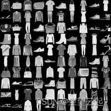

  （7）波士顿房价回归数据集

        Keras 数据集中的另一个可用数据集是波士顿房价回归数据集。 顾名思义，这个数据集可以用于回归，这与我们在这篇博文中已经看到的许多与分类相关的数据集相反。

        加载数据很容易，就像几乎所有的 Keras 数据集一样：

from tensorflow.keras.datasets import boston_housing
(x_train, y_train), (x_test, y_test) = boston_housing.load_data()

        该数据集包含 506 个观察结果，这些观察结果将某些特征与波士顿某个时期的房价（以 1000 美元计）相关联。 正如我们所见：

'''
  Generate a BoxPlot image to determine how many outliers are within the Boston Housing Pricing Dataset.
'''
from tensorflow.keras.datasets import boston_housing
import numpy as np
import matplotlib.pyplot as plt
from scipy import stats as st

# Load the data
(x_train, y_train), (x_test, y_test) = boston_housing.load_data()

# We only need the targets, but do need to consider all of them
y = np.concatenate((y_train, y_test))

# Describe statistics
stats = st.describe(y)
print(stats)

# Generate box plot
plt.boxplot(y)
plt.title('Boston housing price regression dataset - boxplot')
plt.savefig('./boxplot.jpg')

        这些是数据集中存在的所有变量

• CRIM per capita crime rate by town
• ZN proportion of residential land zoned for lots over 25,000 sq.ft.
• INDUS proportion of non-retail business acres per town
• CHAS Charles River dummy variable (= 1 if tract bounds river; 0 otherwise)
• NOX nitric oxides concentration (parts per 10 million)
• RM average number of rooms per dwelling
• AGE proportion of owner-occupied units built prior to 1940
• DIS weighted distances to five Boston employment centres
• RAD index of accessibility to radial highways
• TAX full-value property-tax rate per $10,000
• PTRATIO pupil-teacher ratio by town
• B 1000(Bk - 0.63)^2 where Bk is the proportion of blacks by town
• LSTAT % lower status of the population
• MEDV Median value of owner-occupied homes in $1000'