Python中的图像处理（第九章）Python图像增强

前言

随着人工智能研究的不断兴起，Python的应用也在不断上升，由于Python语言的简洁性、易读性以及可扩展性，特别是在开源工具和深度学习方向中各种神经网络的应用，使得Python已经成为最受欢迎的程序设计语言之一。由于完全开源，加上简单易学、易读、易维护、以及其可移植性、解释性、可扩展性、可扩充性、可嵌入性：丰富的库等等，自己在学习与工作中也时常接触到Python，这个系列文章的话主要就是介绍一些在Python中常用一些例程进行仿真演示！

本系列文章主要参考杨秀章老师分享的代码资源，杨老师博客主页是Eastmount，杨老师兴趣广泛，不愧是令人膜拜的大佬，他过成了我理想中的样子，希望以后有机会可以向他请教学习交流。

因为自己是做图像语音出身的，所以结合《Python中的图像处理》，学习一下Python，OpenCV已经在Python上进行了多个版本的维护，所以相比VS，Python的环境配置相对简单，缺什么库直接安装即可。本系列文章例程都是基于Python3.8的环境下进行，所以大家在进行借鉴的时候建议最好在3.8.0版本以上进行仿真。本文继续来对本书第九章的5个例程进行介绍。

一. Python准备

如何确定自己安装好了python

win+R输入cmd进入命令行程序

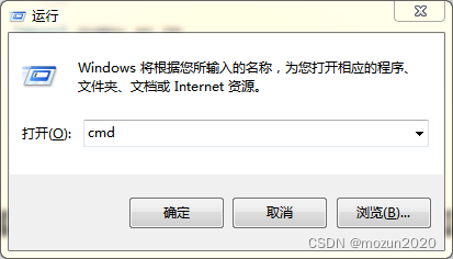
点击“确定”

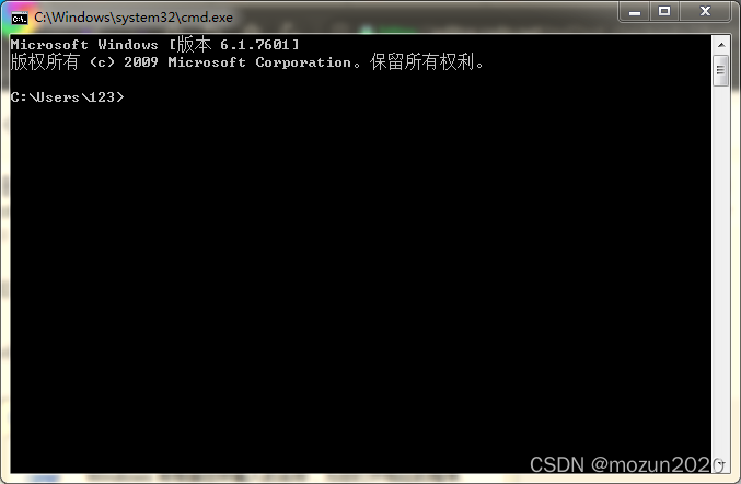
输入：python，回车

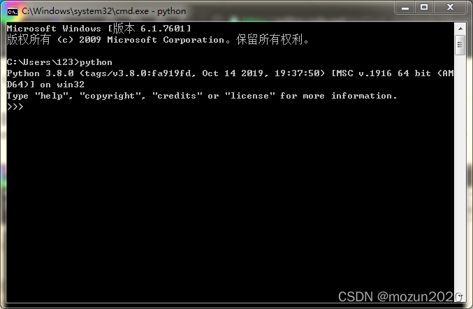
看到Python相关的版本信息，说明Python安装成功。

二. Python仿真

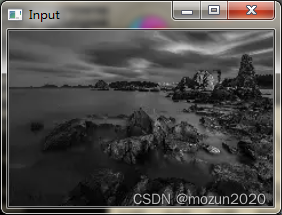
（1）新建一个chapter09_01.py文件，输入以下代码，图片也放在与.py文件同级文件夹下

# -*- coding: utf-8 -*-
# By:Eastmount CSDN 2021-03-12
import cv2  
import numpy as np  
import matplotlib.pyplot as plt
 
#读取图片
img = cv2.imread('test.png')

#灰度转换
gray = cv2.cvtColor(img, cv2.COLOR_BGR2GRAY)
 
#直方图均衡化处理
result = cv2.equalizeHist(gray)

#显示图像
cv2.imshow("Input", gray)
cv2.imshow("Result", result)
cv2.waitKey(0)
cv2.destroyAllWindows()

保存.py文件
输入eixt()退出python，输入命令行进入工程文件目录

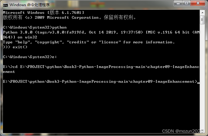
输入以下命令，跑起工程

python chapter09_01.py

没有报错，直接弹出图片，运行成功！


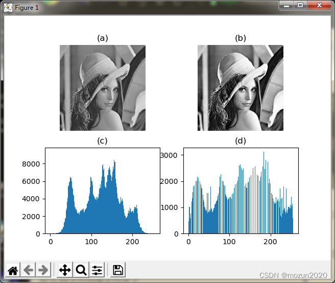
（2）新建一个chapter09_02.py文件，输入以下代码，图片也放在与.py文件同级文件夹下

# -*- coding: utf-8 -*-
# By:Eastmount CSDN 2021-03-12
import cv2  
import numpy as np  
import matplotlib.pyplot as plt
 
#读取图片
img = cv2.imread('lena.bmp')

#灰度转换
gray = cv2.cvtColor(img, cv2.COLOR_BGR2GRAY)
 
#直方图均衡化处理
result = cv2.equalizeHist(gray)

#显示图像
plt.subplot(221)
plt.imshow(gray, cmap=plt.cm.gray), plt.axis("off"), plt.title('(a)') 
plt.subplot(222)
plt.imshow(result, cmap=plt.cm.gray), plt.axis("off"), plt.title('(b)') 
plt.subplot(223)
plt.hist(img.ravel(), 256), plt.title('(c)') 
plt.subplot(224)
plt.hist(result.ravel(), 256), plt.title('(d)') 
plt.show()

保存.py文件输入以下命令，跑起工程

python chapter09_02.py

没有报错，直接弹出图片，运行成功！

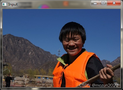
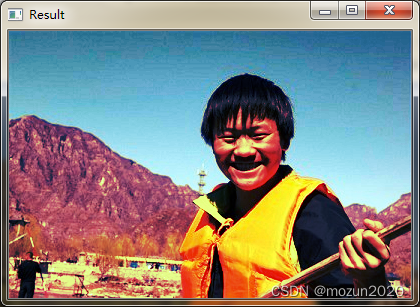
（3）新建一个chapter09_03.py文件，输入以下代码，图片也放在与.py文件同级文件夹下

# -*- coding: utf-8 -*-
# By:Eastmount CSDN 2021-03-12
import cv2  
import numpy as np  
import matplotlib.pyplot as plt

#读取图片
img = cv2.imread('yxz.jpg')

# 彩色图像均衡化 需要分解通道 对每一个通道均衡化
(b, g, r) = cv2.split(img)
bH = cv2.equalizeHist(b)
gH = cv2.equalizeHist(g)
rH = cv2.equalizeHist(r)

# 合并每一个通道
result = cv2.merge((bH, gH, rH))
cv2.imshow("Input", img)
cv2.imshow("Result", result)

#等待显示
cv2.waitKey(0)
cv2.destroyAllWindows()

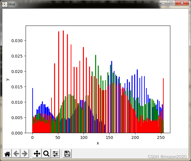
#绘制直方图
plt.figure("Hist")
#蓝色分量
plt.hist(bH.ravel(), bins=256, density=True, facecolor='b', edgecolor='b')
#绿色分量
plt.hist(gH.ravel(), bins=256, density=True, facecolor='g', edgecolor='g')
#红色分量
plt.hist(rH.ravel(), bins=256, density=True, facecolor='r', edgecolor='r')
plt.xlabel("x")
plt.ylabel("y")
plt.show()

保存.py文件输入以下命令，跑起工程

python chapter09_03.py

没有报错，直接弹出图片，运行成功！

（4）新建一个chapter09_04.py文件，输入以下代码，图片也放在与.py文件同级文件夹下

# -*- coding: utf-8 -*-
# By:Eastmount CSDN 2021-03-12
import cv2  
import numpy as np  
import matplotlib.pyplot as plt
 
#读取图片
img = cv2.imread('lena.bmp')

#灰度转换
gray = cv2.cvtColor(img, cv2.COLOR_BGR2GRAY)
 
#局部直方图均衡化处理
clahe = cv2.createCLAHE(clipLimit=2, tileGridSize=(10,10))

#将灰度图像和局部直方图相关联, 把直方图均衡化应用到灰度图 
result = clahe.apply(gray)

#显示图像
plt.subplot(221)
plt.imshow(gray, cmap=plt.cm.gray), plt.axis("off"), plt.title('(a)') 
plt.subplot(222)
plt.imshow(result, cmap=plt.cm.gray), plt.axis("off"), plt.title('(b)') 
plt.subplot(223)
plt.hist(img.ravel(), 256), plt.title('(c)') 
plt.subplot(224)
plt.hist(result.ravel(), 256), plt.title('(d)') 
plt.show()

保存.py文件输入以下命令，跑起工程

python chapter09_04.py

没有报错，直接弹出图片，运行成功！

（5）新建一个chapter09_05.py文件，输入以下代码，图片也放在与.py文件同级文件夹下

# -*- coding: utf-8 -*-
# By:Eastmount CSDN 2021-03-12
# 参考zmshy2128老师文章
import cv2
import numpy as np
import math
import matplotlib.pyplot as plt

#线性拉伸处理
#去掉最大最小0.5%的像素值 线性拉伸至[0,1]
def stretchImage(data, s=0.005, bins = 2000):   
    ht = np.histogram(data, bins);
    d = np.cumsum(ht[0])/float(data.size)
    lmin = 0; lmax=bins-1
    while lmin<bins:
        if d[lmin]>=s:
            break
        lmin+=1
    while lmax>=0:
        if d[lmax]<=1-s:
            break
        lmax-=1
    return np.clip((data-ht[1][lmin])/(ht[1][lmax]-ht[1][lmin]), 0,1)

#根据半径计算权重参数矩阵
g_para = {
    
    }
def getPara(radius = 5):                        
    global g_para
    m = g_para.get(radius, None)
    if m is not None:
        return m
    size = radius*2+1
    m = np.zeros((size, size))
    for h in range(-radius, radius+1):
        for w in range(-radius, radius+1):
            if h==0 and w==0:
                continue
            m[radius+h, radius+w] = 1.0/math.sqrt(h**2+w**2)
    m /= m.sum()
    g_para[radius] = m
    return m

#常规的ACE实现
def zmIce(I, ratio=4, radius=300):                     
    para = getPara(radius)
    height,width = I.shape
    
    #Python3报错 列表append
    """
    #TypeError: can only concatenate list (not "range") to list
    #增加max
    print(range(height),type(range(height)))
    print([0]*radius,type([0]*radius))
    print([height-1]*radius,type([height-1]*radius))
    zh = [0]*radius + max(range(height)) + [height-1]*radius
    zw = [0]*radius + max(range(width))  + [width -1]*radius
    #[0,0,0] + [0,1,2,3] + [3,3,3]
    #[0, 0, 0, 0, 1, 2, 3, 3, 3, 3]
    """

    zh = []
    zw = []
    n = 0
    while n < radius:
        zh.append(0)
        zw.append(0)
        n += 1
    for n in range(height):
        zh.append(n)
    for n in range(width):
        zw.append(n)
    n = 0
    while n < radius:
        zh.append(height-1)
        zw.append(width-1)
        n += 1

    #print(zh)
    #print(zw)
    
    Z = I[np.ix_(zh, zw)]
    res = np.zeros(I.shape)
    for h in range(radius*2+1):
        for w in range(radius*2+1):
            if para[h][w] == 0:
                continue
            res += (para[h][w] * np.clip((I-Z[h:h+height, w:w+width])*ratio, -1, 1))
    return res

#单通道ACE快速增强实现
def zmIceFast(I, ratio, radius):
    #print(I)
    height, width = I.shape[:2]
    if min(height, width) <=2:
        return np.zeros(I.shape)+0.5
    Rs = cv2.resize(I, (int((width+1)/2), int((height+1)/2)))
    Rf = zmIceFast(Rs, ratio, radius)             #递归调用
    Rf = cv2.resize(Rf, (width, height))
    Rs = cv2.resize(Rs, (width, height))
 
    return Rf+zmIce(I,ratio, radius)-zmIce(Rs,ratio,radius)   

#rgb三通道分别增强 ratio是对比度增强因子 radius是卷积模板半径          
def zmIceColor(I, ratio=1, radius=5):               
    res = np.zeros(I.shape)
    for k in range(3):
        res[:,:,k] = stretchImage(zmIceFast(I[:,:,k], ratio, radius))
    return res

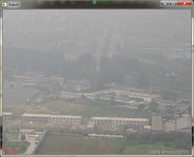
#主函数
if __name__ == '__main__':
    img = cv2.imread('test02.png')
    res = zmIceColor(img/255.0)*255
    cv2.imwrite('Ice.jpg', res)
    
    cv2.imshow("Input", img)
    cv2.imshow("Result", res)
    #等待显示
    cv2.waitKey(0)
    cv2.destroyAllWindows()

保存.py文件输入以下命令，跑起工程

python chapter09_05.py

没有报错，直接弹出图片，运行成功，但算法实现有待优化，显示效果需要调整，后期有时间会进行深入研究跟进！

三. 小结

本文主要介绍在Python中调用OpenCV库对图像进行图像增强，前两个示例可以看到和一般P图软件中的滤镜效果类似，主要就是通过直方图均衡化的方法进行操作的。由于本书的介绍比较系统全面，所以会出一个系列文章进行全系列仿真实现，感兴趣的还是建议去原书第九章深入学习理解，下一篇文章将继续介绍第十章节的5例仿真实例。每天学一个Python小知识，大家一起来学习进步阿！

本系列示例主要参考杨老师GitHub源码，安利一下地址：ImageProcessing-Python（喜欢记得给个star哈！）