RepLKNet实战

摘要
论文解读
安装包
- 1、安装timm
- 2、安装apex
数据增强Cutout和Mixup
项目结构
计算mean和std
生成数据集

摘要

本文通过对植物幼苗分类的实际例子来感受一下超大核的魅力所在。这篇文章能让你学到：

通过对论文的解读，了解RepLKNet超大核的设计思想和架构。
如何使用数据增强，包括transforms的增强、CutOut、MixUp、CutMix等增强手段？
如何调用自定义的模型？
如何使用混合精度训练？
如何使用梯度裁剪防止梯度爆炸？
如何使用DP多显卡训练？
如何绘制loss和acc曲线？
如何生成val的测评报告？
如何编写测试脚本测试测试集？
如何使用余弦退火策略调整学习率？

论文解读

pytoch代码：https://github.com/DingXiaoH/RepLKNet-pytorch

论文翻译：https://wanghao.blog.csdn.net/article/details/124875771?spm=1001.2014.3001.5502

RepLKNet的作者受vision transformers (ViT) 最新进展的启发,提出了31×31的超大核模型，与小核 CNN 相比，大核 CNN 具有更大的有效感受野和更高的形状偏差而不是纹理偏差。借鉴 Swin Transformer 的宏观架构，提出了一种架构 RepLKNet。在 ImageNet 上获得 87.8% 的 top-1 准确率，在 ADE20K 上获得 56.0% mIoU，这在具有相似模型大小的最先进技术中非常具有竞争力。

论文的贡献

论文的主要贡献有：

总结了使用超大核的五条准则：
- 用 depth-wise 超大卷积，最好再加底层优化。
- 加 shortcut
- 用小卷积核做重参数化
- 要看下游任务的性能，不能只看 ImageNet 点数高低
- 小 feature map 上也可以用大卷积，常规分辨率就能训大 kernel 模型
基于以上准则，简单借鉴 Swin Transformer 的宏观架构，我们提出了一种架构 RepLKNet，其中大量使用超大卷积，如 27x27、31x31 等。这一架构的其他部分非常简单，都是 1x1 卷积、Batch Norm 等喜闻乐见的简单结构，不用任何 attention。
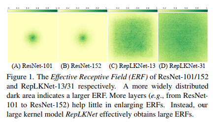
基于超大卷积核，对有效感受野、shape bias（模型做决定的时候到底是看物体的形状还是看局部的纹理？）、Transformers 之所以性能强悍的原因等话题的讨论和分析。我们发现，ResNet-152 等传统深层小 kernel 模型的有效感受野其实不大，大 kernel 模型不但有效感受野更大而且更像人类（shape bias 高），Transformer 可能关键在于大 kernel 而不在于 self-attention 的具体形式。

挑战传统认知

RepLKNet的出现，打破了大家对CNN的固有的认知，主要有：

超大卷积不但不涨点，而且还掉点？RepLKNet证明，超大卷积在过去没人用，不代表其现在不能用。在现代 CNN 设计（shortcut、重参数化等）的加持下，kernel size 越大越涨点！
超大卷积效率很差？超大 depth-wise 卷积并不会增加多少 FLOPs。如果再加点底层优化，速度会更快，31x31 的计算密度最高可达 3x3 的 70 倍！
大卷积只能用在大 feature map 上？作者发现，在 7x7 的 feature map 上用 13x13 卷积都能涨点。
ImageNet 点数说明一切？我们发现，下游（目标检测、语义分割等）任务的性能可能跟 ImageNet 关系不大。
超深 CNN（如 ResNet-152）堆叠大量 3x3，所以感受野很大？作者发现，深层小 kernel 模型有效感受野其实很小。反而少量超大卷积核的有效感受野非常大。
Transformers（ViT、Swin 等）在下游任务上性能强悍，是因为 self-attention（Query-Key-Value 的设计形式）本质更强？作者用超大卷积核验证，发现kernel size 可能才是下游涨点的关键。

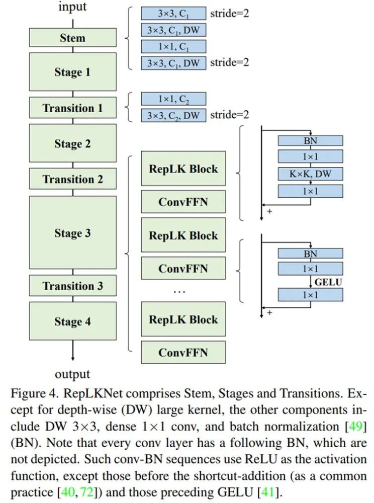
整体架构

作者也说了，架构就是用了Swin Transformer ，主要在于把 attention 换成超大卷积和与之配套的结构，再加一点 CNN 风格的改动。根据以上五条准则，RepLKNet 的设计元素包括 shortcut、depth-wise 超大 kernel、小 kernel 重参数化等。整体架构如下：

下面我们通过对植物幼苗分类的实际例子来感受一下超大核的魅力所在。

安装包

1、安装timm

使用pip就行，命令：

pip install timm

2、安装apex

下载apex库，链接： https://github.com/NVIDIA/apex，下载到本地文件夹。解压后进入到apex的目录安装依赖。在执行命令；

cd C:\Users\XX\Downloads\apex-master #进入apex目录
pip install -r requirements.txt

依赖安装完后，打开cmd，cd进入到刚刚下载完的apex-master路径下，运行：

python setup.py install

数据增强Cutout和Mixup

为了提高成绩我在代码中加入Cutout和Mixup这两种增强方式。实现这两种增强需要安装torchtoolbox。安装命令：

pip install torchtoolbox

Cutout实现，在transforms中。

from torchtoolbox.transform import Cutout
# 数据预处理
transform = transforms.Compose([
    transforms.Resize((224, 224)),
    Cutout(),
    transforms.ToTensor(),
    transforms.Normalize([0.5, 0.5, 0.5], [0.5, 0.5, 0.5])

])

需要导入包：from timm.data.mixup import Mixup，

定义Mixup，和SoftTargetCrossEntropy

  mixup_fn = Mixup(
    mixup_alpha=0.8, cutmix_alpha=1.0, cutmix_minmax=None,
    prob=0.1, switch_prob=0.5, mode='batch',
    label_smoothing=0.1, num_classes=12)
 criterion_train = SoftTargetCrossEntropy()

参数详解：

mixup_alpha (float): mixup alpha 值，如果 > 0，则 mixup 处于活动状态。

cutmix_alpha (float)：cutmix alpha 值，如果 > 0，cutmix 处于活动状态。

cutmix_minmax (List[float])：cutmix 最小/最大图像比率，cutmix 处于活动状态，如果不是 None，则使用这个 vs alpha。

如果设置了 cutmix_minmax 则cutmix_alpha 默认为1.0

prob (float): 每批次或元素应用 mixup 或 cutmix 的概率。

switch_prob (float): 当两者都处于活动状态时切换cutmix 和mixup 的概率。

mode (str): 如何应用 mixup/cutmix 参数（每个’batch’，‘pair’（元素对），‘elem’（元素）。

correct_lam (bool): 当 cutmix bbox 被图像边框剪裁时应用。 lambda 校正

label_smoothing (float)：将标签平滑应用于混合目标张量。

num_classes (int): 目标的类数。

项目结构

RepLKNet_demo
├─data
│  ├─Black-grass
│  ├─Charlock
│  ├─Cleavers
│  ├─Common Chickweed
│  ├─Common wheat
│  ├─Fat Hen
│  ├─Loose Silky-bent
│  ├─Maize
│  ├─Scentless Mayweed
│  ├─Shepherds Purse
│  ├─Small-flowered Cranesbill
│  └─Sugar beet
├─models
│  ├─__init__.py
│  └─replknet.py
├─RepLKNet-31B_ImageNet-1K_224.pth
├─mean_std.py
├─makedata.py
├─train.py
└─test.py

mean_std.py：计算mean和std的值。

makedata.py：生成数据集。

replknet.py:来自官方的pytorch版本的代码。

RepLKNet-31B_ImageNet-1K_224.pth：预训练权重。

计算mean和std

为了使模型更加快速的收敛，我们需要计算出mean和std的值，新建mean_std.py,插入代码：

from torchvision.datasets import ImageFolder
import torch
from torchvision import transforms

def get_mean_and_std(train_data):
    train_loader = torch.utils.data.DataLoader(
        train_data, batch_size=1, shuffle=False, num_workers=0,
        pin_memory=True)
    mean = torch.zeros(3)
    std = torch.zeros(3)
    for X, _ in train_loader:
        for d in range(3):
            mean[d] += X[:, d, :, :].mean()
            std[d] += X[:, d, :, :].std()
    mean.div_(len(train_data))
    std.div_(len(train_data))
    return list(mean.numpy()), list(std.numpy())

if __name__ == '__main__':
    train_dataset = ImageFolder(root=r'data1', transform=transforms.ToTensor())
    print(get_mean_and_std(train_dataset))

数据集结构：

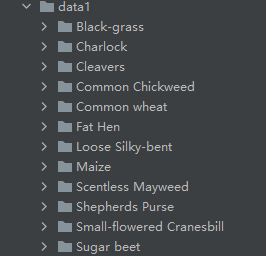
运行结果：

([0.3281186, 0.28937867, 0.20702125], [0.09407319, 0.09732835, 0.106712654])

把这个结果记录下来，后面要用！

生成数据集

我们整理还的图像分类的数据集结构是这样的

data
├─Black-grass
├─Charlock
├─Cleavers
├─Common Chickweed
├─Common wheat
├─Fat Hen
├─Loose Silky-bent
├─Maize
├─Scentless Mayweed
├─Shepherds Purse
├─Small-flowered Cranesbill
└─Sugar beet

pytorch和keras默认加载方式是ImageNet数据集格式，格式是

├─data
│  ├─val
│  │   ├─Black-grass
│  │   ├─Charlock
│  │   ├─Cleavers
│  │   ├─Common Chickweed
│  │   ├─Common wheat
│  │   ├─Fat Hen
│  │   ├─Loose Silky-bent
│  │   ├─Maize
│  │   ├─Scentless Mayweed
│  │   ├─Shepherds Purse
│  │   ├─Small-flowered Cranesbill
│  │   └─Sugar beet
│  └─train
│      ├─Black-grass
│      ├─Charlock
│      ├─Cleavers
│      ├─Common Chickweed
│      ├─Common wheat
│      ├─Fat Hen
│      ├─Loose Silky-bent
│      ├─Maize
│      ├─Scentless Mayweed
│      ├─Shepherds Purse
│      ├─Small-flowered Cranesbill
│      └─Sugar beet

新增格式转化脚本makedata.py,插入代码：

import glob
import os
import shutil

image_list=glob.glob('data1/*/*.png')
print(image_list)
file_dir='data'
if os.path.exists(file_dir):
    print('true')
    #os.rmdir(file_dir)
    shutil.rmtree(file_dir)#删除再建立
    os.makedirs(file_dir)
else:
    os.makedirs(file_dir)

from sklearn.model_selection import train_test_split
trainval_files, val_files = train_test_split(image_list, test_size=0.3, random_state=42)
train_dir='train'
val_dir='val'
train_root=os.path.join(file_dir,train_dir)
val_root=os.path.join(file_dir,val_dir)
for file in trainval_files:
    file_class=file.replace("\\","/").split('/')[-2]
    file_name=file.replace("\\","/").split('/')[-1]
    file_class=os.path.join(train_root,file_class)
    if not os.path.isdir(file_class):
        os.makedirs(file_class)
    shutil.copy(file, file_class + '/' + file_name)

for file in val_files:
    file_class=file.replace("\\","/").split('/')[-2]
    file_name=file.replace("\\","/").split('/')[-1]
    file_class=os.path.join(val_root,file_class)
    if not os.path.isdir(file_class):
        os.makedirs(file_class)
    shutil.copy(file, file_class + '/' + file_name)

完成上面的内容就可以开启训练和测试了，详见下面的链接：

RepLKNet实战：使用RepLKNet实现对植物幼苗的分类（非官方）