Python数据特征分析_01(定基,环比增长,时间序列,标准差等等）

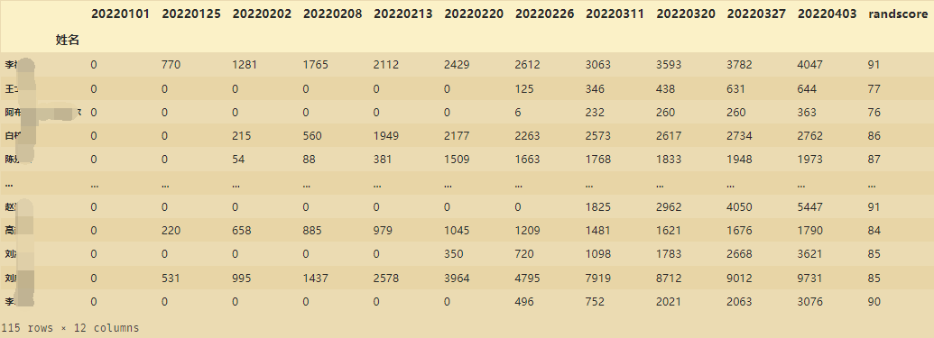
本篇博客使用到的数据如下：通过分析每个学生的学习时长来分析学生的学习稳定性。
（共有115人，每个人记录了11次的学习数据）

一、分布分析

1、定量数据分布分析

定量数据分布分析：主要是求极差

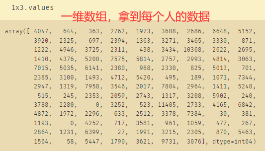
将Excel数据导入之后赋值给x，令x3为最后一周的数据：

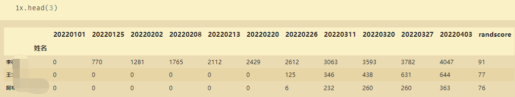
x3=x['20220403']

# 01.求极差
R=x3.max()-x3.min() 
# 得到的极差值：11405

# 02.分桶
rg=np.ceil(R/600)
# 使用600作为分组的间隔
#　np.ceil用法：求出大于等于Ｒ／600的最小整数

得到的rg=20.0，因此如果我们按照间隔600来分组的话，应该要分20桶。

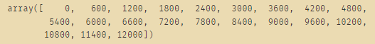
# 构造区间，决定分点
listBins=np.arange(0,12001,600) # 从0-12000，使用600来间隔
listBins

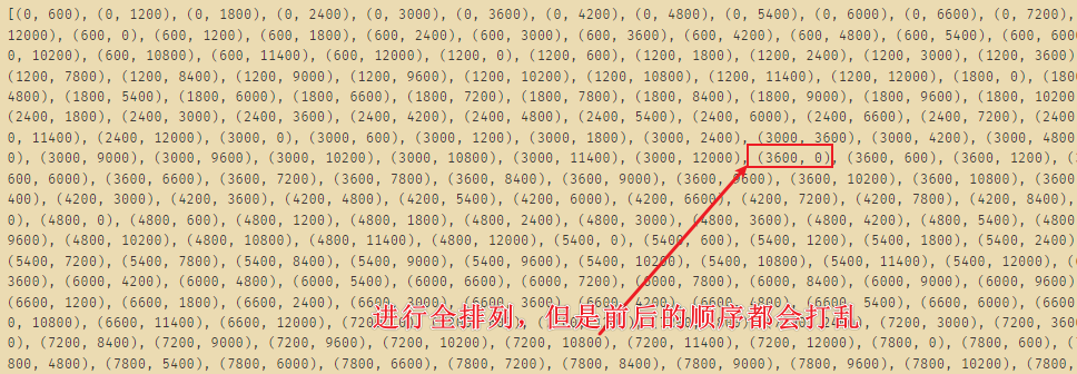
import itertools # 容器工具，根据需要组件特定的数据
aa=listBins
bb=list(itertools.permutations(aa,2))
print(bb)
# python 全排列，permutations函数
# itertools.permutations(iterable, r=None)
# 连续返回由 iterable 元素生成长度为 r 的排列。

fw=list(listBins)
fenzu=pd.cut(x3.values,fw,right=False)
print(fenzu.codes)

print(fenzu.categories)
# IntervalIndex([[0, 600), [600, 1200), [1200, 1800), [1800, 2400), [2400, 3000) ... [9000, 9600), [9600, 10200), [10200, 10800), [10800, 11400), [11400, 12000)], dtype='interval[int64, left]')

ps=fenzu.value_counts()
ps

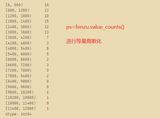
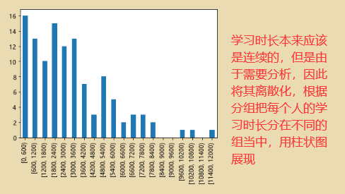
ps.plot(kind='bar')

通过分桶的列表了解学生的学习情况：

qujian=pd.cut(x3,fw,right=False)
x['区间']=qujian.values
x.groupby('区间').median() 		# 获取中位值
x.groupby('区间').mean() 		# 获取平均值
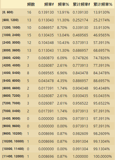
ps_df=pd.DataFrame(ps,columns=['频数'])
ps_df['频率f']=ps_df/ps_df['频数'].sum()
ps_df['频率%']=ps_df['频率f'].map(lambda x:'%.2f%%'%(x*100))
ps_df['累计频率f']=ps_df['频率f'].cumsum() # 累计
ps_df['累计频率%']=ps_df['累计频率f'].map(lambda x:'%.4f%%'%(x*100))
ps_df

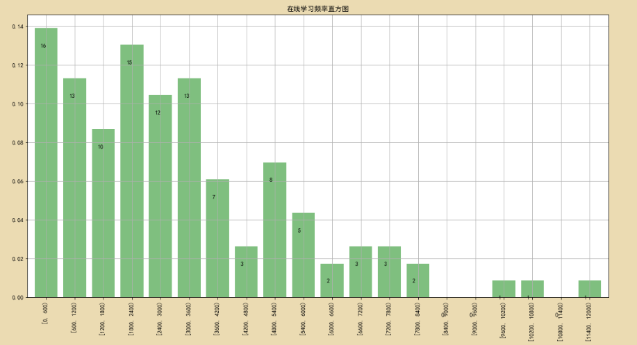
2、绘制频率图

ps_df['频率f'].plot(kind='bar',
                 width=0.8,
                 figsize=(18,9),
                 rot=90,
                 color='g',
                 grid=True,
                 alpha=0.5
                 )
plt.title("在线学习频率直方图")
x=len(ps_df)
y=ps_df['频率f']
m=ps_df['频数']
for i,j,k in zip(range(x),y,m): # 打包函数，将数据重新整合
    plt.text(i-0.2,j-0.01,'%i' % k,color='k') # 代表柱状图上面的数字与柱状图的距离

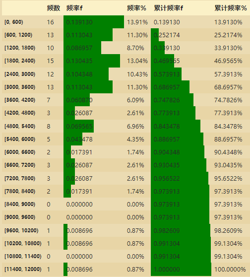
# 类似Excel的对比图
ps_df.style.bar(subset=['频率f','累计频率f'], color='green',width=100)

二、对比分析

1、绝对数对比

import seaborn as sns
import numpy as np
import pandas as pd
import matplotlib as mpl
import matplotlib.pyplot as plt
%matplotlib inline
plt.rcParams['font.sans-serif']=['Microsoft YaHei'] # 用来正常显示中文标签
plt.rcParams['axes.unicode_minus']=False # 用来正常显示负号
from datetime import datetime

fig,axes = plt.subplots(2,1,figsize = (30,20),sharex=False)
dfddiff.plot(kind='line',style='--.',alpha=0.8,ax=axes[0])
axes[0].legend(loc='best',frameon=True,ncol=3)

dfdiffv2.plot(kind='line',style='--.',alpha=0.8,ax=axes[1])
x=range(len(dfdiffv2))
plt.xticks(x,(dfdiffv2.index.values))
axes[1].set_xticklabels(dfdiffv2.index.values,rotation=90)

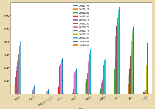
将前10人的数据做bar图：可以分析他们在不同时间段的表现情况

ax=df[0:10].plot(kind='bar',legend=False,figsize=(12,8))
patches,labels=ax.get_legend_handles_labels()
ax.legend(patches,labels,loc='best')
plt.xticks(rotation=30)

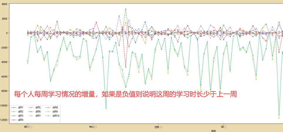
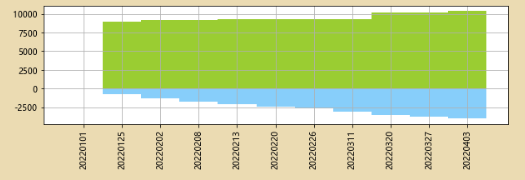
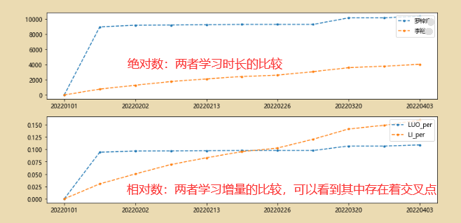
2、差值折线图

# 将两个人的学习时长数据进行比较
fig=plt.figure(figsize=(10,6))
plt.subplots_adjust(hspace=0.3)
ax1=fig.add_subplot(2,1,1)
x=range(len(df2))
y1=df2['罗梓']
y2=-df2['李裕']
plt.bar(x,y1,width=1,facecolor='yellowgreen')
plt.bar(x,y2,width=1,facecolor='lightskyblue')
plt.grid()
plt.xticks(x,(df2.index.values))
ax1.set_xticklabels(df2.index.values,rotation=90)

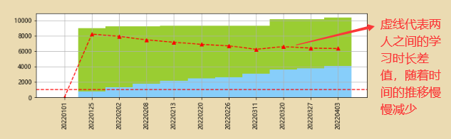
#差值折线图比较
fig=plt.figure(figsize=(10,6))
plt.subplots_adjust(hspace=0.3)
ax1=fig.add_subplot(2,1,1)
x=range(len(df2))
y1=df2['罗梓']
y2=df2['李裕']
y3=y1-y2
plt.plot(x,y3,'--^r')
plt.axhline(1000,color='r',linestyle='--')
plt.bar(x,y1,width=1,facecolor='yellowgreen')
plt.bar(x,y2,width=1,facecolor='lightskyblue')
plt.grid()
plt.xticks(x,(df2.index.values))
ax1.set_xticklabels(df2.index.values,rotation=90)

3、相对数对比

df2['LUO_per']=df2['罗梓']/df2['罗梓'].sum()
df2['LI_per']=df2['李裕']/df2['李裕'].sum()

df2['LUO_per%']=df2['LUO_per'].apply(lambda x:'%.2f%%' %(x*100))
df2['LI_per%']=df2['LI_per'].apply(lambda x:'%.2f%%' %(x*100))

fig,axes=plt.subplots(2,1,figsize=(12,6))
df2[['罗梓','李裕']].plot(kind='line',style='--.',ax=axes[0])
df2[['LUO_per','LI_per']].plot(kind='line',style='--.',ax=axes[1])
axes[0].legend(loc='upper right')
axes[1].legend(loc='upper right')

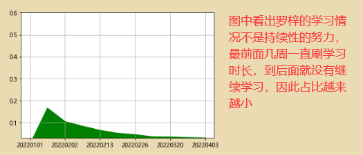
4、比例分析

# 新增df2['totals']列，让其等于所有人每周学习时长的总和。
df2['totals']=df2.iloc[:,0:115].apply(lambda x:x.sum(),axis=1)

# 看看罗梓每周在总学习时长当中所占的比例
df2['LUO_per']=df2['罗梓']/df2['totals']
df2['LUO_per'].plot.area(color='g',ylim=[0.03,0.6],grid=True)

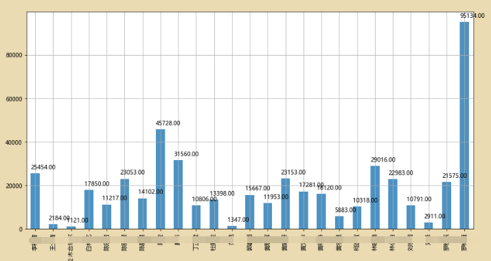
5、空间比较分析

表示利用bar图去看学习时长的高度

plt.figure(figsize=(24,10))
df2.iloc[:,0:25].sum().astype(float).plot(kind = 'bar', alpha = 0.8, grid = True,) 
for i,j in zip(range(115),df2.iloc[:,0:25].sum().astype(float)):
    plt.text(i-0.25,j+2000,'%.2f' % j, color = 'k')

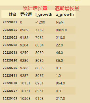
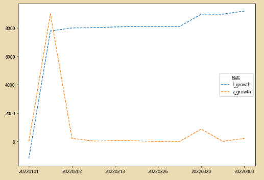
6、动态比较分析

设定1200分钟的学习时长作为及格线

df2['base']=1200
df2.head()

#计算累积增长量和逐期增长量
df2['l_growth']=df2['罗梓烜']-df2['base'] # 与1200相比较
df2['z_growth']=df2['罗梓烜']-df2.shift(1)['罗梓烜']# shift(1)是把数据向下移动1位

df2[['罗梓烜','l_growth','z_growth']]

df3=df2.fillna(0)
df3[['l_growth','z_growth']].plot(figsize=(10,7),style='--')

df2['lspeed']=df2['l_growth']/1200  #定基增长速度
df2['zspeed']=df2['z_growth']/df2.shift(1)['罗梓烜']  #环比增长速度
df2[['lspeed','zspeed']].plot(figsize=(20,10),style='--')

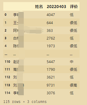
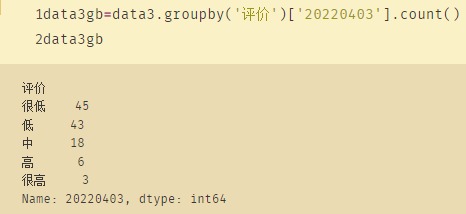
根据学习时长进行评价：
import pandas as pd
data=df.copy() 
label=['很低','低','中','高','很高']
k=5
data2=data['20220403'].copy()  #函数中一定要使用data！！！去改函数
pingjia=pd.cut(data2,k,labels=label)
data3=pd.DataFrame(data2).reset_index().merge((pd.DataFrame(pingjia).reset_index()).rename(columns={
    
    '20220403':'评价'}))
data3

import pandas as pd
import matplotlib.pyplot as plt
%matplotlib inline
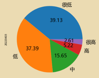
plt.figure(figsize=(10,10))
data3gb.plot.pie(y='x',
                 labels=label, # 标签，指定项目名称
#                  colors=['r', 'g', 'b', 'c','y'], # 指定颜色
                 autopct='%.2f', # 数字格式
                 fontsize=20, # 字体大小
                 figsize=(6, 6) # 图大小
                )

三、统计量分析

集中趋势分析：均值，中位数，众数
离中趋势分析：标准差，变异系数，四分位间距

import numpy as np
import pandas as pd
import matplotlib.pyplot as plt
%matplotlib inline

dfsta=df[['20220403']].copy()
dfsta['f']=np.random.rand(115)
dfsta['f2']=dfsta['20220403']/(dfsta['20220403'].sum())
dfsta
mean=dfsta['20220403'].mean()
mean

#加权平均数
mean_w=(dfsta['20220403']*dfsta['f']).sum()/dfsta['f'].sum()
print('加权平均数是：%.2f' %mean_w)

# 位置平均数
m = dfsta['20220403'].mode()
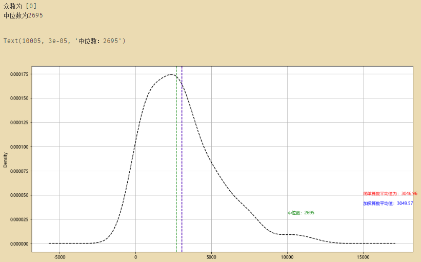
print('众数为',m.tolist())
# 众数是一组数据中出现次数最多的数，这里可能返回多个值

plt.figure(figsize=(16, 8)) 
med = dfsta['20220403'].median()
print('中位数为%i' % med)
# 中位数指将总体各单位标志按照大小顺序排列后，中间位置的数字

dfsta['20220403'].plot(kind = 'kde',style = '--k',grid = True)
# 密度曲线

plt.axvline(mean,color='r',linestyle="--",alpha=0.8)  
plt.text(15000 + 5,0.00005,'简单算数平均值为：%.2f' % mean, color = 'r')
# # 简单算数平均值

plt.axvline(mean_w,color='b',linestyle="--",alpha=0.8)  
plt.text(15000 + 5,0.00004,'加权算数平均值：%.2f' % mean_w, color = 'b',)
# # 加权算数平均值

plt.axvline(med,color='g',linestyle="--",alpha=0.8)  
plt.text(10000 + 5,0.00003,'中位数：%i' % med, color = 'g',)
# 中位数

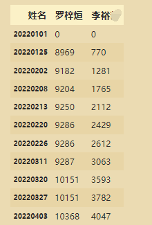
选取两位学生进行比较：

data=df2[['罗梓烜','李裕']].copy()
data

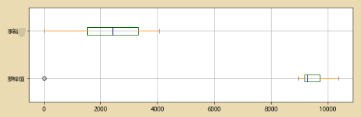
#计算极差
a_r=data['罗梓烜'].max()-data['罗梓烜'].min()
b_r=data['李裕普'].max()-data['李裕普'].min()
print('WU的极差:%.2f,LAI的极差:%.2f' %(a_r,b_r))
print('---------------')
#计算分位差
sta=data['罗梓烜'].describe()
stb=data['李裕普'].describe()
print(sta)
# print(type(sta))
print(stb)
a_iqr = sta.loc['75%'] - sta.loc['25%'] 
b_iqr = stb.loc['75%'] - stb.loc['25%']
print('WU的分位差为：%.2f, LAI的分位差为：%.2f' % (a_iqr,b_iqr))
print('------')
color = dict(boxes='DarkGreen', whiskers='DarkOrange', medians='DarkBlue', caps='Gray')
data.plot.box(vert=False,grid = True,color = color,figsize = (10,3))

# 方差与标准差
a_std = sta.loc['std']
b_std = stb.loc['std']
a_var = data['罗梓烜'].var()
b_var = data['李裕'].var()
print('LUO的标准差为：%.2f, LUO的标准差为：%.2f' % (a_std,b_std))
print('LI的标准差为：%.2f, LI的方差为：%.2f' % (a_var,b_var))
# 方差 → 各组中数值与算数平均数离差平方的算术平均数
# 标准差 → 方差的平方根
# 标准差是最常用的离中趋势指标 → 标准差越大，离中趋势越明显

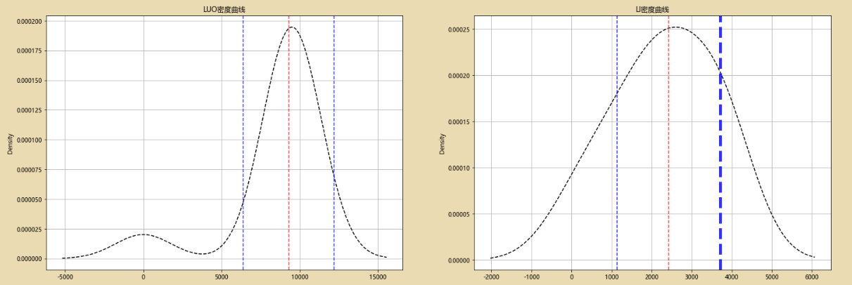
fig = plt.figure(figsize = (24,8))
ax1 = fig.add_subplot(1,2,1)
data['罗梓烜'].plot(kind = 'kde',style = 'k--',grid = True,title = 'LUO密度曲线')
plt.axvline(sta.loc['50%'],color='r',linestyle="--",alpha=0.8)  
plt.axvline(sta.loc['50%'] - a_std,color='b',linestyle="--",alpha=0.8)  
plt.axvline(sta.loc['50%'] + a_std,color='b',linestyle="--",alpha=0.8)  
# A密度曲线，1个标准差

ax2 = fig.add_subplot(1,2,2)
data['李裕'].plot(kind = 'kde',style = 'k--',grid = True,title = 'LI密度曲线')
plt.axvline(stb.loc['50%'],color='r',linestyle="--",alpha=0.8)  
plt.axvline(stb.loc['50%'] - b_std,color='b',linestyle="--",alpha=0.8)  
plt.axvline(stb.loc['50%'] + b_std,color='b',linestyle="--",alpha=0.8,linewidth=5)  
# B密度曲线，1个标准差