Python告诉你三体人有多惨

三体星人非常幸运有两颗恒星，所以他们的生活非常悲惨。

设两颗恒星的质量分别为$M_1,M_2$，而行星的质量对于恒星而言可忽略不计，那么这两颗恒星的运动方程是可以近似为解析解的，而且是高中水平的解析解。

设二者的初始位置是$(-x_1,0),(x_2,0)$，令$L=x_1+x_2$，则$\frac{x_1}{x_2}=\frac{M_2}{M_1}$，记$\mu =\frac{M_2}{M_1}$，则$x_1=\mu x_2$，从而$x_2=\frac{L}{\mu +1},x_1=\frac{\mu L}{\mu +1}$。由于$x_1,x_2$一会儿要用于坐标变量，所以将二者初始位置记为

$$(-\frac{\mu L}{\mu +1},0)(\frac{L}{\mu +1},0)$$

从而二者的角速度为$\omega =\frac{1}{L}\sqrt{\frac{G{M}_1}{x_2}}=\sqrt{\frac{G(M_1+M_2)}{L^3}}$，则二者逆时针旋转，其与$x$轴夹角随时间的变化过程为

$$\begin{gathered} {\theta }_1=\pi +\omega t \\ {\theta }_2=\omega t \end{gathered}$$

转化为直角坐标

$$\begin{array}{rlrl}{x}_2& =\frac{L}{\mu +1}\cos \omega t& x_1& =-\frac{\mu L}{\mu +1}\cos \omega t=-\mu x_2\\ y_2& =\frac{L}{\mu +1}\sin \omega t& y_1& =-\frac{\mu L}{\mu +1}\sin \omega t=-\mu y_2\\ \omega & =\sqrt{\frac{G(M_1+M_2)}{L^3}}& & \end{array}$$

其中，距离单位为千米，当时间单位不同时，万有引力常数为

$$\begin{array}{rl}G& =6.67\times 10^{-11}N\cdot m^2/k{g}^2\\ & =6.67\times 10^{-11}{m}^3{s}^{-2}k{g}^{-1}\\ & =4.98\times 10^{-10}k{m}^3{d}^{-2}k{g}^{-1}\end{array}$$

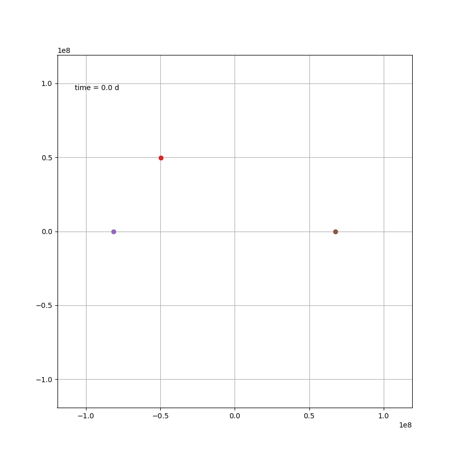
这部分内容不存在任何技术上的问题，如果$\mu =1.2$，则可得如图所示

代码为：

import numpy as np
import scipy.integrate as integrate
import matplotlib.pyplot as plt
import matplotlib.animation as animation

G = 4.98e-10   #时间单位为天
M1 = 2e30  
mu = 1.2
M2 = mu*M1
L = 1.49e8      #km
om = np.sqrt(G*(M1+M2)/L**3)

dt = 2
t = np.arange(0, 250, dt)

x2 = L/(mu+1)*np.cos(om*t)
y2 = L/(mu+1)*np.sin(om*t)
x1,y1 = -mu*x2, -mu*y2

# 下面为绘图过程
fig = plt.figure(figsize=(9,9))
ax = fig.add_subplot(111, autoscale_on=False, 
    xlim=(-0.8*L, 0.8*L), ylim=(-0.8*L, 0.8*L))
ax.grid()

line1, = ax.plot([], [], lw=2)
line2, = ax.plot([], [], lw=2)
time_template = 'time = %.1f d'
time_text = ax.text(0.05, 0.9, '', transform=ax.transAxes)

def animate(i):
    line1.set_data(x1[:i],y1[:i])
    line2.set_data(x2[:i],y2[:i])
    time_text.set_text(time_template % (i*dt))
    return line1, line2, time_text

ani = animation.FuncAnimation(fig, animate, range(len(t)),   
        interval=10, blit=True)
ani.save("tri_1.gif",writer='imagemagick')
plt.show()

现在，假设有一颗不知死活的行星闯入了二星世界，若其所在位置是$(x,y)$，质量为$m$，则其动能为

$$T=\frac{1}{2}m({\dot{x}}^2+{\dot{y}}^2)$$

引力势能为

$$V=-\frac{G{M}_{1}m}{\sqrt{(x-x_1{)}^2+(y-y_1{)}^2}}-\frac{G{M}_{2}m}{\sqrt{(x-x_2{)}^2+(y-y_2{)}^2}}$$

拉格朗日量为$L=T-V$，根据拉格朗日方程

$$\frac{\text{d}}{\text{d}t}\frac{\partial L}{\partial \dot{r}}-\frac{\partial L}{\partial r}=0，r=x,y$$

有

$$\begin{gathered} \ddot{x}=\frac{G{M}_1(x-x_1)}{{\sqrt{(x-x_1{)}^2+(y-y_1{)}^2}}^3}+\frac{G{M}_2(x-x_2)}{{\sqrt{(x-x_2{)}^2+(y-y_2{)}^2}}^3} \\ \ddot{y}=\frac{G{M}_1(y-y_1)}{{\sqrt{(x-x_1{)}^2+(y-y_1{)}^2}}^3}+\frac{G{M}_2(y-y_2)}{{\sqrt{(x-x_2{)}^2+(y-y_2{)}^2}}^3} \end{gathered}$$

其微分方程写为

# 其中，mu,G,M1,M2为全局变量
def derivs(state, t):
    dydx = np.zeros_like(state)
    x, vx, y, vy = state
    x2 = L/(mu+1)*np.cos(om*t)
    y2 = L/(mu+1)*np.sin(om*t)
    x1 = -mu*x2
    y1 = -mu*y2
    L1 = np.sqrt((x-x1)**2+(y-y1)**2)**3
    L2 = np.sqrt((x-x2)**2+(y-y2)**2)**3
    dydx[0] = state[1]
    dydx[1] = -G*(M1*(x-x1)/L1+M2*(x-x2)/L2)
    dydx[2] = state[3]
    dydx[3] = -G*(M1*(y-y1)/L1+M2*(y-y2)/L2)
    return dydx

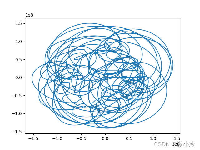
接下来根据微分方程的解，便可进行绘图，假设上帝把这颗行星轻轻地放在$(L/4,L/4)$的位置上，那么接下来它的运行轨迹如下

# 星体等数据可按照上面的代码来写
# 生成时间
dt = 1
t = np.arange(0, 250, dt)

x, y = -L/3, L/3
vx0 = 0
vy0 = 0
state = np.array([x,vx0,y,vy0])

# 微分方程组数值解
x,vx,y,vy = integrate.odeint(derivs, state, t).T
plt.plot(x,y)
plt.show()

当然也可以画下动图，可以说非常吊诡了，而这只是一种三体运动形式

x2 = L/(mu+1)*np.cos(om*t)
y2 = L/(mu+1)*np.sin(om*t)
x1 = -mu*x2
y1 = -mu*y2

def animate(i):
    pt0.set_data(x[i],y[i])
    pt1.set_data(x1[i],y1[i])
    pt2.set_data(x2[i],y2[i])
    line0.set_data(x[:i],y[:i])
    line1.set_data(x1[:i],y1[:i])
    line2.set_data(x2[:i],y2[:i])
    time_text.set_text(time_template % (i*dt))
    return line0, line1, line2, pt0, pt1, pt2, time_text

fig = plt.figure(figsize=(9,9))
ax = fig.add_subplot(111, autoscale_on=False, 
    xlim=(-0.8*L, 0.8*L), ylim=(-0.8*L, 0.8*L))
ax.grid()

line0, = ax.plot([], [], lw=2)
line1, = ax.plot([], [], lw=2)
line2, = ax.plot([], [], lw=2)
pt0, = ax.plot([x[0]],[y[0]] ,marker='o')
pt1, = ax.plot([x1[0]],[y1[0]] ,marker='o')
pt2, = ax.plot([x2[0]],[y2[0]] ,marker='o')

time_template = 'time = %.1f d'
time_text = ax.text(0.05, 0.9, '', 
    transform=ax.transAxes)

ani = animation.FuncAnimation(fig, animate, t,   
        interval=0.1, blit=True)
plt.show()
ani.save("tri_3.gif")

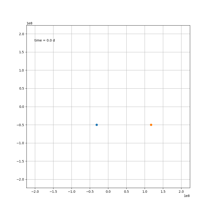
如果站在这颗行星上，去观察另外两颗恒星，那么可能会更加感受到这种压迫感。然而就这个案例来说，除了最开始那一下好像贴上恒星了，后面的状态要比预想中要好一些。然而这只是几百天的运行轨迹，不知道几百万年还会跑出什么花样。总之，三体星能产生个生命也是绝了。

X1,X2 = x1-x,x2-x
Y1,Y2 = y1-y,y2-y

fig = plt.figure(figsize=(9,9))
ax = fig.add_subplot(111, autoscale_on=False, 
    xlim=(-1.5*L, 1.5*L), ylim=(-1.5*L, 1.5*L))
ax.grid()

pt1, = ax.plot([X1[0]],[Y1[0]] ,marker='o')
pt2, = ax.plot([X2[0]],[Y2[0]] ,marker='o')
line1, = ax.plot([], [], lw=2)
line2, = ax.plot([], [], lw=2)
time_template = 'time = %.1f d'
time_text = ax.text(0.05, 0.9, '', transform=ax.transAxes)

def animate(i):
    pt1.set_data(X1[i],Y1[i])
    pt2.set_data(X2[i],Y2[i])
    line1.set_data(X1[:i],Y1[:i])
    line2.set_data(X2[:i],Y2[:i])
    time_text.set_text(time_template % (i*dt))
    return line1, line2, pt1, pt2, time_text

ani = animation.FuncAnimation(fig, animate, range(len(t)),   
        interval=10, blit=True)

ani.save("tri_4.gif",writer='imagemagick')
plt.show()