MobileNetv1、MobileNetv2、MobileNetv3

MobileNetv1
MobileNet的由来：谷歌在2017年提出了，专注于移动端或者嵌入式设备中的轻量级CNN网络，其最大的创新点是，提出了深度可分离卷积（depthwise separable convolution）

论文地址：https://arxiv.org/pdf/1704.04861.pdf

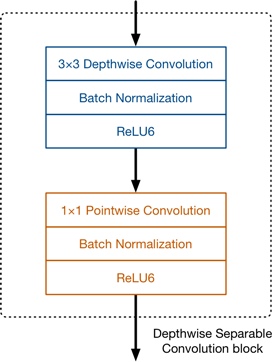
下图显示depthwise separable convolution的合成过程
在这里插入图片描述

分析depthwise separable convolution在计算量上和标准卷积的差别

输入的特征图的大小是： $in_{width} * in_{height} * in_{channel}$
输出的特征图的大小是： $out_{width} * out_{height} * out_{channel}$
卷积核的大小定义为： $k * k$

计算计算量

标准卷积的计算量： $k * k * out_{channel} * in_{channel} * out_{width} * out_{height}$
depthwise convolution的计算量： $k * k * in_{channel} * out_{width} * out_{height}$
pointwise convolution的计算量： $in_{channel} * out_{channel} * out_{width} * out_{height}$
depthwise separable convolution的总计算量：
$k * k * in_{channel} * out_{width} * out_{height} + in_{channel} * out_{channel} * out_{width} * out_{height}$
depthwise separable convolution和标准卷积的比较：
$\frac{k * k * in_{channel} * out_{width} * out_{height} + in_{channel} * out_{channel} * out_{width} * out_{height}}{k * k * out_{channel} * in_{channel} * out_{width} * out_{height}} = \frac{1}{out_{channel}} + \frac{1}{k^2}$

从公式上，我们能看出，如果卷积核的大小为3的时候，depthwise separable convolution 可以降低大约8-9倍的计算量！！！

MobileNetv1的模型架构如下：（左侧是标准卷积；右侧是MobileNetv1卷积模型）
在这里插入图片描述

注意一点：MobileNetV1中使用的ReLU使用的是ReLU6

$R e L U 6 = m i n (m a x (f e a t u r e s, 0), 6)$
在这里插入图片描述
ReLU6和ReLU的对比图

使用ReLU6的目的
主要是为了在移动端float16的低精度的时候，也能有很好的数值分辨率，如果对ReLu的输出值不加限制，那么输出范围就是0到正无穷，而低精度的float16无法精确描述其数值，带来精度损失。

具体的卷积流程
在这里插入图片描述

Mult-Adds：当前模块参与整个网络的计算程度
Parmaeters：当前模型占有整个网络的参数量

说明一点：
MobileNetv1为了提高计算速度，谷歌采用扩大分辨率，减小宽度的方法。
在这里插入图片描述

但是需要注意的是：
在训练过程中，mobileNet的速度大概是VGG的3倍，但是在同样的训练集open image下，mobileNet 的mAP要比VGG低20个点左右。

	(0): Conv2d(128, 128, kernel_size=(3, 3), stride=(2, 2), padding=(1, 1), groups=128, bias=False)
	(1): BatchNorm2d(128, eps=1e-05, momentum=0.1, affine=True, track_running_stats=True)
	(2): ReLU6(inplace=True)
	(3): Conv2d(128, 256, kernel_size=(1, 1), stride=(1, 1), bias=False)
	(4): BatchNorm2d(256, eps=1e-05, momentum=0.1, affine=True, track_running_stats=True)
	(5): ReLU6(inplace=True)

MobileNetv2
论文：《Inverted Residuals and Linear Bottlenecks: Mobile Networks for Classification, Detection and Segmentation》
MobileNetv2相比于MobileNetv1做了两个改进（从论文上不难看出）：Inverted Residuals and Linear Bottlenecks

在这里插入图片描述
从上图中，我们不难看出，MobileNet v2在Depthwise convolution之前添加一层Pointwise convolution

so，为什么添加一层Pointwise convolution？

当加一层Pointwise convolution就可以升维，也可以降维；
在MobileNet v2中加的这一层是用做升维；
Pointwise卷积升维之后，Depthwise卷积就可以在高维度工作。

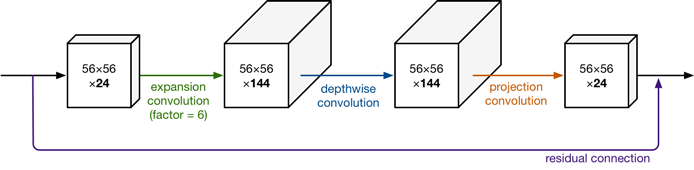
这一层的Pointwise 卷积就可以叫expansion卷积，这一层就可以叫expansion layer，因为它用来升维了。
升了多少倍或者说通道扩大了多少倍就有了expansion factor：144/24=6倍

t：通道扩张倍数
c：输出通道数
n：重复次数
s：stride

Inverted residuals
什么是Inverted residuals？inverted residuals：倒残差

和残差结构的区别如下：
在这里插入图片描述
为什么叫做倒残差呢？

Inverted residual 的实现

 import torch.nn as nn
    
    from torch.nn import functional as F
    
    class InvertedResidual(nn.Module):
    
        def __init__(self, in_features, out_features, stride, expand_ratio,activation=nn.ReLU6) :
            super(InvertedResidual, self).__init__()
            self.stride = stride
            assert stride in [1, 2]
            hidden_dim = in_features * expand_ratio
            self.is_residual = self.stride == 1 and in_features == out_features
            self.conv = nn.Sequential(
                        # pw Point-wise 
                        nn.Conv2d(in_features, hidden_dim, 1, 1, 0, bias=False),
                        nn.BatchNorm2d(hidden_dim),
                        activation(inplace=True),
                        # dw  Depth-wise
                        nn.Conv2d(hidden_dim, hidden_dim, 3, stride, 1, groups=hidden_dim, bias=False),
                        nn.BatchNorm2d(hidden_dim),
                        activation(inplace=True),
                        # pw-linear, Point-wise linear
                        nn.Conv2d(hidden_dim, out_features, 1, 1, 0, bias=False),
                        nn.BatchNorm2d(out_features),
                    )
    
    
        def forward(self, x):
            if self.is_residual:
                return x + self.conv(x)
            else:
                return self.conv(x)
            
       
    print(InvertedResidual(1280, 512, stride=2, expand_ratio=6)  )

Linear bottlenecks
为什么称为瓶颈：
如下图所示，resnet的结构，其结构可以看为是一个花瓶，为此，说到瓶颈（Bottleneck），我们应最先想到ResNet网络结构，mobileNetV2同样使用了该结构。
在这里插入图片描述
其次就是Linear
下图是mobileNetV1和mobileNetV2结构之间的区别

论文中提到：高维加个非线性挺好，低维要是也加非线性就把特征破坏了，不如线性的好，所以1*1后不加ReLU6 ，改换线性。

stride=1

 (conv): Sequential(
        (0): ConvBNReLU(
          (0): Conv2d(24, 144, kernel_size=(1, 1), stride=(1, 1), bias=False)
          (1): BatchNorm2d(144, eps=1e-05, momentum=0.1, affine=True, track_running_stats=True)
          (2): ReLU6(inplace=True)
        )
        (1): ConvBNReLU(
          (0): Conv2d(144, 144, kernel_size=(3, 3), stride=(1, 1), padding=(1, 1), groups=144, bias=False)
          (1): BatchNorm2d(144, eps=1e-05, momentum=0.1, affine=True, track_running_stats=True)
          (2): ReLU6(inplace=True)
        )
        (2): Conv2d(144, 24, kernel_size=(1, 1), stride=(1, 1), bias=False)
        (3): BatchNorm2d(24, eps=1e-05, momentum=0.1, affine=True, track_running_stats=True)
      )

stride=2

InvertedResidual(
  (conv): Sequential(
    (0): Conv2d(1280, 7680, kernel_size=(1, 1), stride=(1, 1), bias=False)
    (1): BatchNorm2d(7680, eps=1e-05, momentum=0.1, affine=True, track_running_stats=True)
    (2): ReLU6(inplace)
    (3): Conv2d(7680, 7680, kernel_size=(3, 3), stride=(2, 2), padding=(1, 1), groups=7680, bias=False)
    (4): BatchNorm2d(7680, eps=1e-05, momentum=0.1, affine=True, track_running_stats=True)
    (5): ReLU6(inplace)
    (6): Conv2d(7680, 512, kernel_size=(1, 1), stride=(1, 1), bias=False)
    (7): BatchNorm2d(512, eps=1e-05, momentum=0.1, affine=True, track_running_stats=True)
  )
)

注意一点：MobileNetv2中stride=1 和 stride=2 走的流程是不同的

stride=1

point-wise升维
depth-wise提取特征
通过Linear的point-wise降维
input与结果相加（残差结构）

区别于stride=2

input与output的大小不同，所以没有添加shortcut结构

思考：mobileNetV2中先利用point-wise进行升维的话会提高许多计算量，是否还支持：深度可分离卷积和轻量化模型？

v2比v1由于多了一层，那参数量确实就变大了，而实际上在v2设计中会把通道变小。 v2通道数不会升维到v1的那么大。

$V_{mobileNetV1} < V_{mobileNetV2}$

MobileNetv3
前面已经说过:

MobileNetV1 模型引入的深度可分离卷积（depthwise separable convolutions);
MobileNetV2 模型引入的具有线性瓶颈的倒残差结构(the inverted residual with linear bottleneck)；

那么MobileNetv3又是什么？
论文链接：https://arxiv.org/abs/1905.02244

MobileNetv3是Google基于MobileNetv2之后的又一个力作，从精度和时间上均有所提高：

MobileNetv3提供了两个版本：分别是mobileNetV3 Large 和 MobileNetV3 Small 分别对应对计算和存储要求高和低的版本。

论文中也提到：
在这里插入图片描述

mobilenet-v3 small在imagenet数据集分类任务上，较mobilenet-v2，精度提高了大约3.2%，时间却减少了15%
mobilenet-v3 large在imagenet数据集分类任务上，较mobilenet-v2，精度提高了大约4.6%，时间减少了5%
mobilenet-v3 large 与v2相比，在COCO数据集上达到相同的精度，速度快了25%

MobileNetV3做了哪些修改呢？

引入了SE结构
修改尾部结构
修改channel的数量
非线性变换的改变

引入了SE结构

SE是什么，全称： $S q u e e z e - a n d - E x c i t e$ 其对应的论文是：《Squeeze-and-Excitation Networks》

SE是一个子模块，可以嵌到其他的模型中

在这里插入图片描述
Sequeeze-and-Excitation的层次结构可以分为两个部分：Sequeeze部分和Excitation部分
Sequeeze部分其实指的是：AdaptiveAvgPool2d
Excitation部分指的是：

Linear
ReLU
Linear
Sigmoid

为此我们也就清楚了SE网络的结构

AdaptiveAvgPool2d
Linear
ReLU
Linear
Sigmoid

在这里插入图片描述

可以用一句话总结SE网络的特性：特征少的抑制它，特征多的就多多关注它。
常见的几种添加注意力(attention)机制：https://www.jianshu.com/p/fcd8991143c8

在这里插入图片描述
修改尾部网络结构
在mobilenetv2中，在avg pooling之前，存在一个1x1的卷积层，目的是提高特征图的维度，更有利于结构的预测，但是这其实带来了一定的计算量了，为此作者首先利用avg pooling将特征图大小由7x7降到了1x1，这样就减少了7x7=49倍的计算量。

并且为了进一步的降低计算量，Google团队直接去掉了前面纺锤型卷积的3x3以及1x1卷积，就变成了如下图第二行所示的结构，Google团队将其中的3x3以及1x1去掉后，精度并没有得到损失。

这里降低了大约15ms的速度。

在这里插入图片描述
修改channel数量
修改头部卷积核channel数量，mobilenet v2中使用的是32 x 3 x 3，作者发现，其实32可以再降低一点，所以这里作者改成了16，在保证了精度的前提下，降低了3ms的速度。

mobilenet v2以及mobilenet v3的结构对比：
在这里插入图片描述

非线性变换的改变
为了提高速度，Google团队提出了一种新的激活函数swish x 能有效改进网络精度：

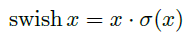
但是sigmoid的计算耗时较长，特别是在移动端，这些耗时就会比较明显

所以作者使用 $\frac{ReLU6(x+3)}{6}$ 来近似替代sigmoid:
在这里插入图片描述
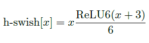
如下两张图展示的是使用h-swish对于时间以及精度的影响，可以发现，使用h-swish@16会导致精度略有提高0.2%，同时增加了近20%的延迟。

下图是将mobilenet v3应用于SSD-Lite在COCO测试集的精度结果

观察可以发现，在V3上面，mAP没有特别大的提升但是延迟确实降低了一些的

在这里插入图片描述

MobileNetv1、MobileNetv2、MobileNetv3

猜你喜欢