
1 introduction
文中,作者研究了如何有效地处理神经推荐系统中的上下文数据。 首先对传统的将上下文作为特征的方法进行了分析,并证明这种方法在捕获特征交叉时效率低下。然后据此来设计RNN推荐系统。 We first describe our RNN-based recommender system in use at YouTube. Next, we offer “Latent Cross,” an easy-to-use technique to incorporate contextual data in the RNN by embedding the context feature first and then performing an element-wise product of the context embedding with model’s hidden states.
学习的目的 to best learn from users actions, e.g., clicks, purchases, watches, and ratings…
一些重要的contextual data:request and watch time, the type of device, and the page on the website or mobile app
2 describe
Netflix Prize setting e ≡ ( i , j , R ) e \equiv(i, j, R) e≡(i,j,R), user i i i gave movie j j j a rating of R R R. e ≡ ( i , j , t , d ) e \equiv(i, j, t, d) e≡(i,j,t,d), user i i i watched video j j j at time t t t on device type d d d.
recommender systems as trying to predict one value of the event given the others: for a tuple e = ( i , j , R ) e = (i, j, R) e=(i,j,R), use ( i , j ) (i, j) (i,j) predict R R R.
Symbol Description e Tuple of k values describing an observed event e ℓ Element ℓ in the tuple E Set of all observed events u i , v j Trainable embeddings of user i and item j X i All events for user i X i , t All events for user i befor time t e ( τ ) Event at step τ in a particular sequence < ⋅ > k way inner product ∗ Element-wise product f ( ⋅ ) An arbitrary neural network \begin{array}{lll}{\text { Symbol }} & {\text { Description }} \\ \hline e & {\text { Tuple of } k \text { values describing an observed event }} \\ {e_{\ell}} & {\text { Element } \ell \text { in the tuple }} \\ {\mathcal{E}} & {\text { Set of all observed events }} \\ {u_{i}, v_{j}} & {\text { Trainable embeddings of user } i \text { and item } j} \\ {X_{i}} & {\text { All events for user } i} \\ {X_{i, t}} & {\text { All events for user i befor time t}} \\ {e^{(\tau)}} & {\text { Event at step } \tau \text { in a particular sequence }} \\ {<·>} & {\text { k way inner product}} \\ {*} & {\text { Element-wise product }} \\ {f(\cdot)} & {\text { An arbitrary neural network }}\end{array} Symbol eeℓEui,vjXiXi,te(τ)<⋅>∗f(⋅) Description Tuple of k values describing an observed event Element ℓ in the tuple Set of all observed events Trainable embeddings of user i and item j All events for user i All events for user i befor time t Event at step τ in a particular sequence k way inner product Element-wise product An arbitrary neural network
machine learning perspective, we can split our tuple e into features x and label y such that x = ( i , j ) and label y = R . \begin{array}{l}{\text { machine learning perspective, we can split our tuple } e \text { into features }} \ {x \text { and label } y \text { such that } x=(i, j) \text { and label } y=R \text { . }}\end{array} machine learning perspective, we can split our tuple e into features x and label y such that x=(i,j) and label y=R .
矩阵分解: u i ⋅ v j u_{i} \cdot v_{j} ui⋅vj
张量分解: ∑ r u i , r v j , r w t , r \sum_{r} u_{i, r} v_{j, r} w_{t, r} ∑rui,rvj,rwt,r
表示称内积: ⟨ u i , v j , w t ⟩ = ∑ r u i , r v j , r w t , r \left\langle u_{i}, v_{j}, w_{t}\right\rangle=\sum_{r} u_{i, r} v_{j, r} w_{t, r} ⟨ui,vj,wt⟩=∑rui,rvj,rwt,r
3 MoDELING PRELIMINARIES
3.1 First Order DNN的局限
模型最后的输出: h τ = g ( W τ h τ − 1 + b τ ) h_{\tau}=g\left(W_{\tau} h_{\tau-1}+b_{\tau}\right) hτ=g(Wτhτ−1+bτ),这个公式可看做 h τ − 1 h_{\tau - 1} hτ−1的一阶转换,原因就是只涉及了 h τ − 1 h_{\tau - 1} hτ−1中元素的加法,并没有涉及到元素间的乘法。
矩阵分解可以捕捉到不同类型输入(user,item,time等)之间的低秩关系
3.2 Modeling Low-Rank Relations
通过生成一些low-rank数据来验证first order DNN是否可以很好的建模low-rank之间的关系。
生成长度为 r r r的随机向量 u i u_i ui : u i ∼ N ( 0 , 1 r 1 / 2 m I ) u_{i} \sim \mathcal{N}\left(0, \frac{1}{r^{1 / 2 m}} \mathbf{I}\right) ui∼N(0,r1/2m1I),其中 r r r为data的秩,m个特征。
当 m = 3 m=3 m=3时,每个样本可以表示成 ( i , j , t , ⟨ u i , u j , u t ⟩ ) \left(i, j, t,\left\langle u_{i}, u_{j}, u_{t}\right\rangle\right) (i,j,t,⟨ui,uj,ut⟩),将三部分合并起来作为输入,然后经过RELU激活函数输入到最终的线性层,损失函数采用MSE( mean squared error loss ),采用Adagrade进行优化 ,最终以Pearson correlation进行评价。
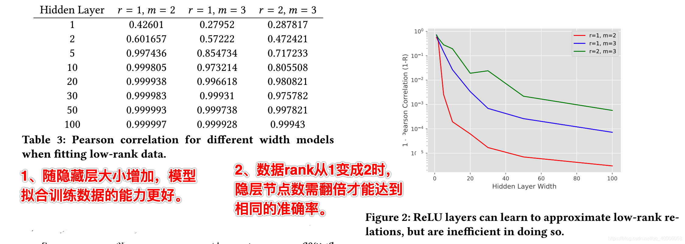
1、随着隐藏层大小增加,模型拟合训练数据的能力更好。
2、rank从1变成2时,隐藏层nodes需要翻倍才能达到相同的准确率。
3、Considering collaborative filtering models will often discover rank 200 relations , this intuitively suggests that real world models would require very wide layers for a single two-way relation to be learned.
结果:ReLU layers越多,拟合的越好,但效率低。因此开始考虑RNN模型。
4 YOUTUBE’S RECURRENT RECOMMENDER
RNNs are notable as a baseline model because they are already second-order neural networks, significantly more complex than the first-order models explored above, and are at the cutting edge of dynamic recommender systems
4.1 Formal Description
the input to the model is the set of events for user: X i = { e = ( i , j , ψ ( j ) , t ) ∈ E ∣ e 0 = i } X_{i}=\left\{e=(i, j, \psi(j), t) \in \mathcal{E} | e_{0}=i\right\} Xi={ e=(i,j,ψ(j),t)∈E∣e0=i}, use X i , t X_{i,t} Xi,t to denote all watches before t t t for user X i X_i Xi : X i , t = { e = ( i , j , t ) ∈ E ∣ e 0 = i ∧ e 3 < t } ⊂ X I X_{i, t}=\left\{e=(i, j, t) \in \mathcal{E} | e_{0}=i \wedge e_{3}<t\right\} \subset X_{I} Xi,t={ e=(i,j,t)∈E∣e0=i∧e3<t}⊂XI, Pr ( j ∣ i , t , X i , t ) \operatorname{Pr}\left(j | i, t, X_{i, t}\right) Pr(j∣i,t,Xi,t) 表示the video j j j that user i i i will watch at a given time t t t based on all watches before t t t.
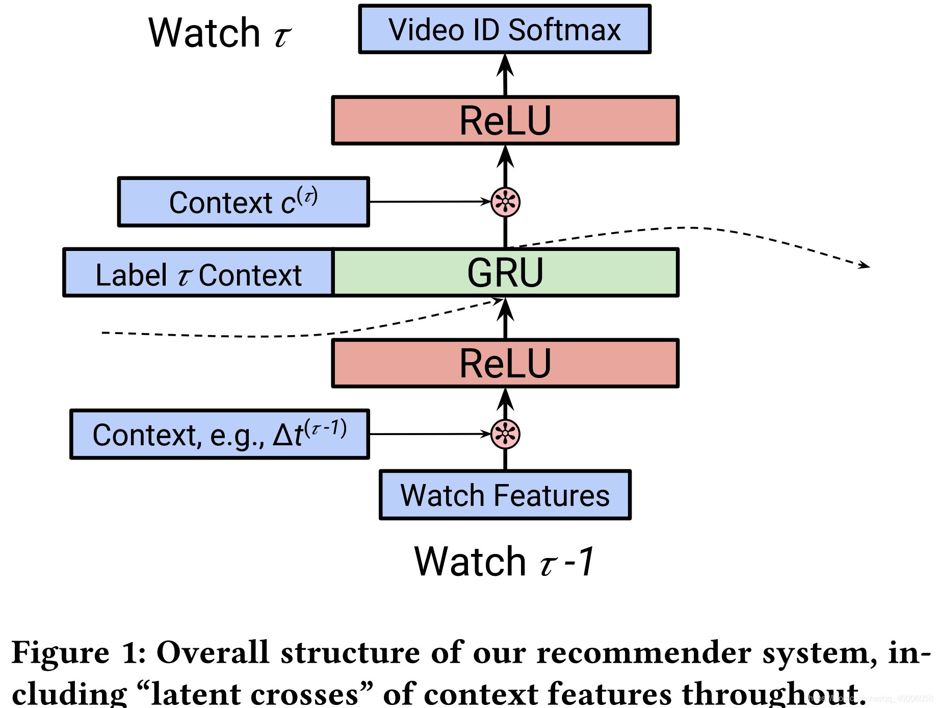
user i i i在time t t t观看 ψ ( j ) \psi(j) ψ(j)上传的具有 w t w_t wt feature的video j j j。模型以user i i i在time t t t之前的浏览记录 X i , t X_{i,t} Xi,t作为输入。使用 e ( τ ) e^{(\tau)} e(τ)表示序列中的第 τ \tau τ次事件, x ( τ ) x^{(\tau)} x(τ)表示事件 e ( τ ) e^{(\tau)} e(τ)转换后的输入(就是user i i i对应的一些embedding),而 y ( τ ) y^{(\tau)} y(τ)表示预测的标签。当前时刻 e ( τ ) = ( i , j , ψ ( j ) , t ) e^{(\tau)}=(i, j, \psi(j), t) e(τ)=(i,j,ψ(j),t) , 下一时刻 e ( τ + 1 ) = ( i , j ′ , ψ ( j ′ ) , t ′ ) e^{(\tau+1)}=\left(i, j^{\prime}, \psi\left(j^{\prime}\right), t^{\prime}\right) e(τ+1)=(i,j′,ψ(j′),t′),则输入 x ( τ ) = [ v j ; u ψ ( j ) ; w t ] x^{(\tau)}=\left[v_{j} ; u_{\psi}(j) ; w_{t}\right] x(τ)=[vj;uψ(j);wt]来预测标签 y ( τ + 1 ) = j ′ y^{(\tau+1)}=j^{'} y(τ+1)=j′,其中 v j v_{j} vj是video的embedding, u ψ ( j ) u_{\psi}(j) uψ(j)是上传者(uploader)的embedding, w t w_{t} wt是情景的embedding。在预测 y ( τ + 1 ) y^{(\tau+1)} y(τ+1)时,不能使用 e ( τ ) e^{(\tau)} e(τ)的标签作为输入,但是可以使用 w t w_{t} wt的情景特征,记为 c ( τ ) = [ w t ] c^{(\tau)}=\left[w_{t}\right] c(τ)=[wt]。
4.2 Structure of the Baseline RNN Model
RNN模型对一系列的actions进行建模:
1、对于每个event e ( τ ) e^{(\tau)} e(τ), e ( τ ) e^{(\tau)} e(τ)对应为 x ( τ ) x^{(\tau)} x(τ),先输入到一层NN中得到 h 0 ( τ ) = f i ( x ( τ ) ) h_{0}^{(\tau)}=f_{i}\left(x^{(\tau)}\right) h0(τ)=fi(x(τ))
2、将其输入到RNN(LSTM、GRU)模型,得到 h 1 ( τ ) , z ( τ ) = f r ( h 0 ( τ ) , z ( τ − 1 ) ) h_{1}^{(\tau)}, z^{(\tau)}=f_{r}\left(h_{0}^{(\tau)}, z^{(\tau-1)}\right) h1(τ),z(τ)=fr(h0(τ),z(τ−1))
3、使用 f o ( h 1 ( τ − 1 ) , c ( τ ) ) f_{o}\left(h_{1}^{(\tau-1)}, c^{(\tau)}\right) fo(h1(τ−1),c(τ))来预测 y ( τ ) y^{(\tau)} y(τ)
4.3 Context Features
1、TimeDelta
Δ t ( τ ) = log ( t ( τ + 1 ) − t ( τ ) ) \Delta t^{(\tau)}=\log \left(t^{(\tau+1)}-t^{(\tau)}\right) Δt(τ)=log(t(τ+1)−t(τ))
2、Software Client
video的长短会影响user观看使用的device
3、Page
从网站home_page开始浏览的话可能对new content更有兴趣,从一个具体的video page跳转可能表示user对某个特定的topic更感兴趣。
4、Pre- and Post-Fusion.
前面将情景特征标记为 c ( τ ) c^{(\tau)} c(τ) ,pre-fusion表示情景特征从NN底部作为input,post-fusion表示和RNN的输出合并起来。把 c ( τ ) − 1 c^{(\tau)-1} c(τ)−1作为pre-fusion特征来影响RNN的state,而把 c ( τ ) c^{(\tau)} c(τ)作为post-fusion特征来直接用于预测 y ( τ ) y^{(\tau)} y(τ)。
5 CONTEXT MODELING WITH THE LATENT CROSS
前面介绍,直接将content feature concat 是低效的,因此下面展开研究。
5.1 Single Feature
以time为例,perform an element-wise product in the middle of the network h 0 ( τ ) = ( 1 + w t ) ∗ h 0 ( τ ) h_{0}^{(\tau)}=\left(1+w_{t}\right) * h_{0}^{(\tau)} h0(τ)=(1+wt)∗h0(τ), 通过 0-mean Gaussian来初始化 w w w,有两点好处:
1、This can be interpreted as the context providing a mask or attention mechanism over the hidden state. (相当于在隐状态上加了mask和attention)
2、enables low-rank relations between the input previous watch and the time.(捕捉上次记录与time的low-rank关系)
对于 h 1 ( τ ) h_{1}^{(\tau)} h1(τ), h 1 ( τ ) = ( 1 + w t ) ∗ h 1 ( τ ) h_{1}^{(\tau)}=\left(1+w_{t}\right) * h_{1}^{(\tau)} h1(τ)=(1+wt)∗h1(τ).
5.2 Using Multiple Features
通常,会有很多 contextual feature,以device和time为例: h ( τ ) = ( 1 + w t + w d ) ∗ h ( τ ) h^{(\tau)}=\left(1+w_{t}+w_{d}\right) * h^{(\tau)} h(τ)=(1+wt+wd)∗h(τ)
1、相当于在隐状态上加了mask和attention
2、捕捉2-way relation
3、加法运算容易训练, 而 w t ∗ w d ∗ h ( τ ) w_{t} * w_{d} * h^{(\tau)} wt∗wd∗h(τ)以及 f ( [ w t ; w d ] ) f\left(\left[w_{t} ; w_{d}\right]\right) f([wt;wd])难训练\。