深度学习入门实验part（上）

加载数据集

在这里插入图片描述
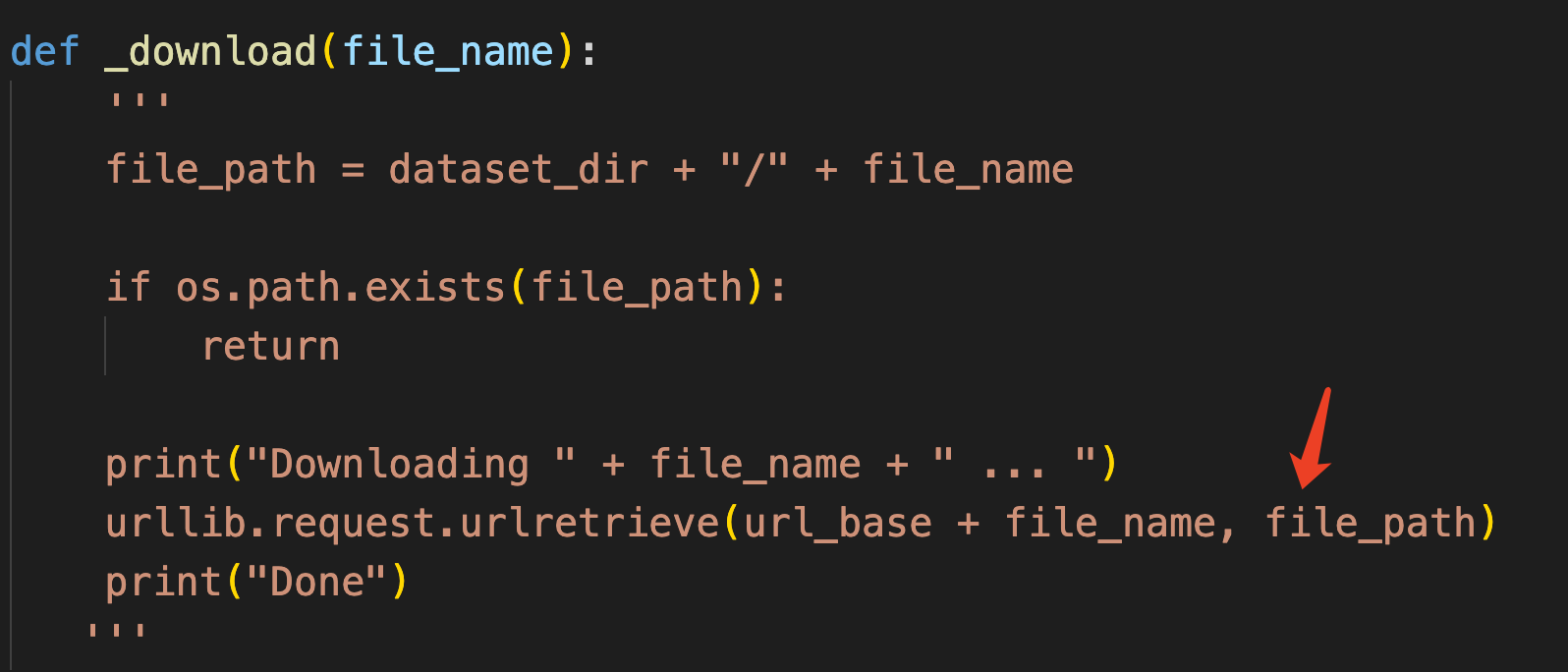
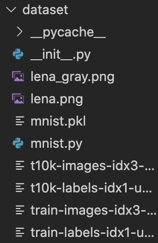
原本的minist.py脚本进入到这一行之后一直报503错误，由于我对爬虫类了解不多，最后选择手动下载了minist数据集，再进行处理。

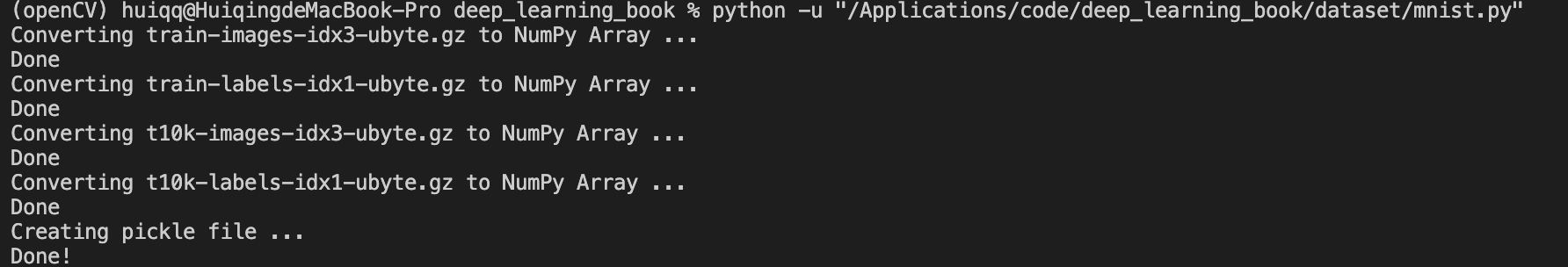
直到这里算是数据加载完成了。

三、神经网络

pickle功能：这个功能可以将程序运行中的对象保存为文件。如果加载保存过的pickle文件，可以立刻复原之前程序中运行的对象。

读取MINST中的数据

不知道是不是sys.path.append(os.pardir)失效了，from dataset.mnist import load_mnist还是不能够找到minist.py，要使用deep_learning_book.dataset.mnist。

import sys, os
sys.path.append(os.pardir)  # 为了导入父目录的文件而进行的设定
import numpy as np
from deep_learning_book.dataset.mnist import load_mnist
from PIL import Image # pickle功能

def img_show(img):  
    pil_img = Image.fromarray(np.uint8(img))#把numpy数组的图像数据转换为PIL的数据对象
    pil_img.show()
    
# (训练图像，训练标签)，（测试图像，测试标签）
(x_train, t_train), (x_test, t_test) = load_mnist(flatten=True, normalize=False)
#还可以有第三个参数,one_hot_label=False 
#eg.tag=3,one-hot表示为tag=[0,0,0,1,0,0,0,0,0,0]
print(x_train.shape) # (60000, 784)  28*28=784
print(t_train.shape) # (60000,)
print(x_test.shape) # (10000, 784)
print(t_test.shape) # (10000,)

img = x_train[0]
label = t_train[0]
print(label)  # 5

print(img.shape)  # (784,)
# flatten=True时，读入的图像是以一维numpy数组存储的，显示图像时要恢复成28*28
img = img.reshape(28, 28)  # 把图像的形状变为原来的尺寸
print(img.shape)  # (28, 28)

img_show(img)

神经网络的推理处理（手写数字的识别）

输入层：784个neuron
隐藏层1：50个neuron （任意设定）
隐藏层2：100个neuron（任意设定）

输入一张图像进行处理：

在这里插入图片描述

print(x.shape)  # (10000, 784)
print(W1.shape) # (784, 50)
print(W2.shape) # (50, 100)
print(W3.shape) # (100, 10)

sample_weight.pkl中以字典变量的形式保存了weight和bias

import sys, os
sys.path.append(os.pardir)  # 为了导入父目录的文件而进行的设定
import numpy as np
import pickle
from deep_learning_book.dataset.mnist import load_mnist
from deep_learning_book.common.functions import sigmoid, softmax


def get_data():
    (x_train, t_train), (x_test, t_test) = load_mnist(normalize=True, flatten=True, one_hot_label=False)
    return x_test, t_test

# 读入保存在sample_weight.pkl中学习到的权重参数
def init_network():
    with open("ch03/sample_weight.pkl", 'rb') as f:
        network = pickle.load(f)
    return network


def predict(network, x): # 用该函数来进行分类
    W1, W2, W3 = network['W1'], network['W2'], network['W3']
    b1, b2, b3 = network['b1'], network['b2'], network['b3']

    a1 = np.dot(x, W1) + b1
    z1 = sigmoid(a1)
    a2 = np.dot(z1, W2) + b2
    z2 = sigmoid(a2)
    a3 = np.dot(z2, W3) + b3
    y = softmax(a3)

    return y  # 返回0~9这十个数字的概率


x, t = get_data()
network = init_network()
accuracy_cnt = 0
for i in range(len(x)):
    y = predict(network, x[i])
    p= np.argmax(y) # 获取概率最高的元素的索引
    if p == t[i]:
        accuracy_cnt += 1

print("Accuracy:" + str(float(accuracy_cnt) / len(x)))

批处理

打包输入多张图像，进行并行处理：
在这里插入图片描述

x, t = get_data()
network = init_network()

batch_size = 100 # 批数量
accuracy_cnt = 0

for i in range(0, len(x), batch_size):
    x_batch = x[i:i+batch_size]
    y_batch = predict(network, x_batch)
    p = np.argmax(y_batch, axis=1)
    accuracy_cnt += np.sum(p == t[i:i+batch_size])

print("Accuracy:" + str(float(accuracy_cnt) / len(x)))

参数axis=1 指定了在100*10的数组中，沿着第1维方向找到值最大的元素的索引。

np.sum(y==t) 用来统计数组中为True的元素个数。

import numpy as np 
x=np.array([[0.1,0.8,0.1],
            [0.3,0.1,0.6],
            [0.2,0.5,0.3],
            [0.8,0.1,0.1]])
y=np.argmax(x,axis=1)
print(y)
# [1 2 1 0]
t=np.array([1,2,0,0])
print(y==t) # [ True  True False  True]
ans=np.sum(y==t)
print(ans) # 3

四、神经网络的学习

梯度

$f(x_0,x_1)=x_0^2+x_1^2$ 的梯度法更新过程：

在这里插入图片描述

import numpy as np
import matplotlib.pylab as plt
from gradient_2d import numerical_gradient

def gradient_descent(f, init_x, lr=0.01, step_num=100):
    x = init_x
    x_history = []

    for i in range(step_num):
        x_history.append( x.copy() )

        grad = numerical_gradient(f, x)
        x -= lr * grad

    return x, np.array(x_history)

def function_2(x):
    return x[0]**2 + x[1]**2

init_x = np.array([-3.0, 4.0])    

lr = 0.1
step_num = 20
x, x_history = gradient_descent(function_2, init_x, lr=lr, step_num=step_num)

plt.plot( [-5, 5], [0,0], '--b')
plt.plot( [0,0], [-5, 5], '--b')
plt.plot(x_history[:,0], x_history[:,1], 'o')

plt.xlim(-3.5, 3.5)
plt.ylim(-4.5, 4.5)
plt.xlabel("X0")
plt.ylabel("X1")
plt.show()

神经网络的梯度

# functions
import numpy as np
def identity_function(x):
    return x
def step_function(x):
    return np.array(x > 0, dtype=np.int)
def sigmoid(x):
    return 1 / (1 + np.exp(-x))    
def sigmoid_grad(x):
    return (1.0 - sigmoid(x)) * sigmoid(x)
def relu(x):
    return np.maximum(0, x)
def relu_grad(x):
    grad = np.zeros(x)
    grad[x>=0] = 1
    return grad
def softmax(x):
    if x.ndim == 2:
        x = x.T
        x = x - np.max(x, axis=0)
        y = np.exp(x) / np.sum(np.exp(x), axis=0)
        return y.T 

    x = x - np.max(x) # 溢出对策
    return np.exp(x) / np.sum(np.exp(x))

def mean_squared_error(y, t):
    return 0.5 * np.sum((y-t)**2)

def cross_entropy_error(y, t):
    if y.ndim == 1:
        t = t.reshape(1, t.size)
        y = y.reshape(1, y.size)
        
    # 监督数据是one-hot-vector的情况下，转换为正确解标签的索引
    if t.size == y.size:
        t = t.argmax(axis=1)
             
    batch_size = y.shape[0]
    return -np.sum(np.log(y[np.arange(batch_size), t] + 1e-7)) / batch_size

def softmax_loss(X, t):
    y = softmax(X)
    return cross_entropy_error(y, t)

# gradient
import numpy as np
def _numerical_gradient_1d(f, x):
    h = 1e-4 # 0.0001
    grad = np.zeros_like(x)
    
    for idx in range(x.size):
        tmp_val = x[idx]
        x[idx] = float(tmp_val) + h
        fxh1 = f(x) # f(x+h)
        
        x[idx] = tmp_val - h 
        fxh2 = f(x) # f(x-h)
        grad[idx] = (fxh1 - fxh2) / (2*h)
        
        x[idx] = tmp_val # 还原值
        
    return grad

def numerical_gradient_2d(f, X):
    if X.ndim == 1:
        return _numerical_gradient_1d(f, X)
    else:
        grad = np.zeros_like(X)
        
        for idx, x in enumerate(X):
            grad[idx] = _numerical_gradient_1d(f, x)
        
        return grad

def numerical_gradient(f, x):
    h = 1e-4 # 0.0001
    grad = np.zeros_like(x)
    
    it = np.nditer(x, flags=['multi_index'], op_flags=['readwrite'])
    while not it.finished:
        idx = it.multi_index
        tmp_val = x[idx]
        x[idx] = float(tmp_val) + h
        fxh1 = f(x) # f(x+h)
        
        x[idx] = tmp_val - h 
        fxh2 = f(x) # f(x-h)
        grad[idx] = (fxh1 - fxh2) / (2*h)
        
        x[idx] = tmp_val # 还原值
        it.iternext()          
    return grad

import sys, os
sys.path.append(os.pardir)  # 为了导入父目录中的文件而进行的设定
import numpy as np
from deep_learning_book.common.functions import softmax, cross_entropy_error
from deep_learning_book.common.gradient import numerical_gradient
class simpleNet:
    def __init__(self):
        self.W = np.random.randn(2,3)

    def predict(self, x):
        return np.dot(x, self.W)

    def loss(self, x, t):
        z = self.predict(x)
        y = softmax(z)
        loss = cross_entropy_error(y, t)

        return loss

x = np.array([0.6, 0.9])
t = np.array([0, 0, 1])

net = simpleNet()
f = lambda w: net.loss(x, t)
dW = numerical_gradient(f, net.W)
print(dW)
# [[ 0.10221412  0.11690908 -0.2191232 ]
#  [ 0.15332117  0.17536362 -0.32868479]]

学习算法的实现（随机梯度下降法）

抽取mini-batch（目标是减小mini-batch的损失函数的值）
计算梯度（为了减小mini-batch的损失函数的值而求各个权重参数的梯度，梯度表示损失函数的值减小最多的方向）
更新参数（权重参数沿梯度方向进行微小更新）
重复上述步骤

# TwoLayerNet类的实现
import sys, os
sys.path.append(os.pardir)  # 为了导入父目录的文件而进行的设定
from deep_learning_book.common.functions import *
from deep_learning_book.common.gradient import numerical_gradient
class TwoLayerNet:

    def __init__(self, input_size, hidden_size, output_size, weight_init_std=0.01):
        # 初始化权重
        # weight使用符合高斯分布的随机数进行初始化，bias用0进行初始化
        self.params = {
    
    }
        self.params['W1'] = weight_init_std * np.random.randn(input_size, hidden_size) # 第一层的weight
        self.params['b1'] = np.zeros(hidden_size) # 第一层的bias
        self.params['W2'] = weight_init_std * np.random.randn(hidden_size, output_size) # 第二层的wight
        self.params['b2'] = np.zeros(output_size) # 第二层的bias

    def predict(self, x): # x是图像数据，进行正向识别（推理）
        W1, W2 = self.params['W1'], self.params['W2']
        b1, b2 = self.params['b1'], self.params['b2']
    
        a1 = np.dot(x, W1) + b1
        z1 = sigmoid(a1)
        a2 = np.dot(z1, W2) + b2
        y = softmax(a2)
        
        return y
        
    # x:输入数据, t:监督数据
    def loss(self, x, t): # x是图像数据，t是正确解标签，进行损失函数值的计算
        y = self.predict(x)    
        return cross_entropy_error(y, t)
    
    def accuracy(self, x, t): # 计算识别精度
        y = self.predict(x)
        y = np.argmax(y, axis=1)
        t = np.argmax(t, axis=1)
        
        accuracy = np.sum(y == t) / float(x.shape[0])
        return accuracy
        
    # x:输入数据, t:监督数据
    def numerical_gradient(self, x, t): # 计算权重参数的梯度
        loss_W = lambda W: self.loss(x, t)
        
        grads = {
    
    }
        grads['W1'] = numerical_gradient(loss_W, self.params['W1']) # 第一层weight的梯度
        grads['b1'] = numerical_gradient(loss_W, self.params['b1']) # 第一层bias的梯度
        grads['W2'] = numerical_gradient(loss_W, self.params['W2'])
        grads['b2'] = numerical_gradient(loss_W, self.params['b2'])
        
        return grads
        
    def gradient(self, x, t): # 用误差反向传播高效计算梯度
        W1, W2 = self.params['W1'], self.params['W2']
        b1, b2 = self.params['b1'], self.params['b2']
        grads = {
    
    }
        
        batch_num = x.shape[0]
        
        # forward
        a1 = np.dot(x, W1) + b1
        z1 = sigmoid(a1)
        a2 = np.dot(z1, W2) + b2
        y = softmax(a2)
        
        # backward
        dy = (y - t) / batch_num
        grads['W2'] = np.dot(z1.T, dy)
        grads['b2'] = np.sum(dy, axis=0)
        
        da1 = np.dot(dy, W2.T)
        dz1 = sigmoid_grad(a1) * da1
        grads['W1'] = np.dot(x.T, dz1)
        grads['b1'] = np.sum(dz1, axis=0)

        return grads

基于测试数据的评价

在这里插入图片描述
通过反复学习可以使损失函数对训练数据的某个mini-batch的损失函数逐渐减小，我们还需要确认在其他数据集上也有同等程度的表现，需要判断是否会出现过拟合。

神经网络学习的最初目标是掌握泛化能力（即必须使用不包含在训练数据中的数据），这里我们通过定期(一个epoch)记录训练数据和测试数据的识别精度来进行观察。（没必要每次记录，只要掌握大致趋势即可，所以用epoch）

一个epoch表示学习中所有训练数据均被使用过一次的更新次数。
eg.对于10000个训练数据，用大小为100的mini-batch进行学习时，重复随机梯度下降法进行100次，就可认为所有训练数据都被使用过了，这里的epoch=100。

在这里插入图片描述

随着epoch的前进（学习的进行）识别精度都有提高，且实验结果表明训练精度和测试精度几乎一致，说明没有发生过拟合现象。

import sys, os
sys.path.append(os.pardir)  # 为了导入父目录的文件而进行的设定
import numpy as np
import matplotlib.pyplot as plt
from deep_learning_book.dataset.mnist import load_mnist
from two_layer_net import TwoLayerNet

# 读入数据
(x_train, t_train), (x_test, t_test) = load_mnist(normalize=True, one_hot_label=True)

network = TwoLayerNet(input_size=784, hidden_size=50, output_size=10)

iters_num = 10000  # 适当设定梯度法的更新次数，每更新一次，都对训练数据计算损失函数值，并添加到数组中
train_size = x_train.shape[0]
batch_size = 100 # 每次从60000个训练数据中随机选取100个数据(图像数据和正确解标签)
learning_rate = 0.1

train_loss_list = [] # 用来记录损失函数值
train_acc_list = [] # 用来记录训练数据集的识别精度
test_acc_list = [] # 用来记录测试数据集的识别精度

iter_per_epoch = max(train_size / batch_size, 1) # 每过这么多次梯度下降就进入一个新epoch，minist数据集60000/100=600

for i in range(iters_num): # 循环次数上限10000 /600 =17次输出识别精度
    # 获取mini-batch
    batch_mask = np.random.choice(train_size, batch_size)
    x_batch = x_train[batch_mask]
    t_batch = t_train[batch_mask]
    
    # 用误差反向传播算法高效计算梯度
    #grad = network.numerical_gradient(x_batch, t_batch)
    grad = network.gradient(x_batch, t_batch)
    
    # 更新参数
    for key in ('W1', 'b1', 'W2', 'b2'):
        network.params[key] -= learning_rate * grad[key]
    # 计算损失函数值，并记录在数组中
    loss = network.loss(x_batch, t_batch)
    train_loss_list.append(loss)
    # 计算每个epoch的识别精度，并存储在数组中
    if i % iter_per_epoch == 0:
        train_acc = network.accuracy(x_train, t_train)
        test_acc = network.accuracy(x_test, t_test)
        train_acc_list.append(train_acc)
        test_acc_list.append(test_acc)
        print("train acc, test acc | " + str(train_acc) + ", " + str(test_acc))

# 绘制图形
markers = {
    
    'train': 'o', 'test': 's'} # 设置线条颜色
x = np.arange(len(train_acc_list))
plt.plot(x, train_acc_list, label='train acc')
plt.plot(x, test_acc_list, label='test acc', linestyle='--')
plt.xlabel("epochs")
plt.ylabel("accuracy")
plt.ylim(0, 1.0)
plt.legend(loc='lower right')
plt.show()

五、误差反向传播算法

误差反向传播算法的实现

前提

神经网络中有合适的weight和bias，调整w和b以便拟合训练数据的过程称为学习。分为以下4个步骤：

抽取mini-batch（目标是减小mini-batch的损失函数的值）
计算梯度（为了减小mini-batch的损失函数的值而求各个权重参数的梯度，梯度表示损失函数的值减小最多的方向）
更新参数（权重参数沿梯度方向进行微小更新）
重复上述步骤

# Two_layer_net 组装层版本
import sys, os
sys.path.append(os.pardir)  # 为了导入父目录的文件而进行的设定
import numpy as np
from deep_learning_book.common.layers import *
from deep_learning_book.common.gradient import numerical_gradient
from collections import OrderedDict
class TwoLayerNet:

    def __init__(self, input_size, hidden_size, output_size, weight_init_std = 0.01):
        # 初始化权重
        self.params = {
    
    }
        self.params['W1'] = weight_init_std * np.random.randn(input_size, hidden_size)
        self.params['b1'] = np.zeros(hidden_size)
        self.params['W2'] = weight_init_std * np.random.randn(hidden_size, output_size) 
        self.params['b2'] = np.zeros(output_size)

        # 生成层 
        self.layers = OrderedDict()
        self.layers['Affine1'] = Affine(self.params['W1'], self.params['b1'])
        self.layers['Relu1'] = Relu()
        self.layers['Affine2'] = Affine(self.params['W2'], self.params['b2'])

        self.lastLayer = SoftmaxWithLoss()
        
    def predict(self, x):
        for layer in self.layers.values():
            x = layer.forward(x)       
        return x
        
    # x:输入数据, t:监督数据
    def loss(self, x, t):
        y = self.predict(x)
        return self.lastLayer.forward(y, t)
    
    def accuracy(self, x, t):
        y = self.predict(x)
        y = np.argmax(y, axis=1)
        if t.ndim != 1 : t = np.argmax(t, axis=1)
        
        accuracy = np.sum(y == t) / float(x.shape[0])
        return accuracy
        
    # x:输入数据, t:监督数据
    def numerical_gradient(self, x, t):
        loss_W = lambda W: self.loss(x, t)
        
        grads = {
    
    }
        grads['W1'] = numerical_gradient(loss_W, self.params['W1'])
        grads['b1'] = numerical_gradient(loss_W, self.params['b1'])
        grads['W2'] = numerical_gradient(loss_W, self.params['W2'])
        grads['b2'] = numerical_gradient(loss_W, self.params['b2'])    
        return grads
        
    def gradient(self, x, t): # 用误差反向传播高效计算梯度
        # forward
        self.loss(x, t)

        # backward
        dout = 1
        dout = self.lastLayer.backward(dout)
        
        layers = list(self.layers.values())
        layers.reverse() # 逆序调用各层
        for layer in layers:
            dout = layer.backward(dout)

        # 设定
        grads = {
    
    }
        grads['W1'], grads['b1'] = self.layers['Affine1'].dW, self.layers['Affine1'].db
        grads['W2'], grads['b2'] = self.layers['Affine2'].dW, self.layers['Affine2'].db
        return grads

将神经网络的层保存为OrderedDict(有序字典)，它可以记住向字典里添加元素的顺序。

正向传播只需要按照添加元素的顺序调用各层的forward()方法就可以完成处理
反向传播只需要按照相反的顺序调用各层即可

Affine层和ReLU层内部会正确处理正向传播和反向传播，所以这里要做的仅仅是以正确顺序连接各层，再按顺序(或逆序)调用各层。

这样只需要不断添加必要的层就可以组装新的神经网络了。

使用误差反向传播法的学习

代码同上一节。

梯度确认

基于数值微分的方法numerical_gradient()，简单耗时，不易出错。
解析性地求解数学式，误差反向传播法gradient()，即使存在大量参数，也可以高效计算梯度。

常用数值微分来确认误差反向传播算法的实现是否正确。

# gradient_check
import sys, os
sys.path.append(os.pardir)  # 为了导入父目录的文件而进行的设定
import numpy as np
from deep_learning_book.dataset.mnist import load_mnist
from two_layer_net import TwoLayerNet
# 读入数据
(x_train, t_train), (x_test, t_test) = load_mnist(normalize=True, one_hot_label=True)

network = TwoLayerNet(input_size=784, hidden_size=50, output_size=10)

x_batch = x_train[:3]
t_batch = t_train[:3]

grad_numerical = network.numerical_gradient(x_batch, t_batch)
grad_backprop = network.gradient(x_batch, t_batch)

for key in grad_numerical.keys():
    diff = np.average( np.abs(grad_backprop[key] - grad_numerical[key]) )
    print(key + ":" + str(diff))
# W1:3.2932210651190824e-10
# b1:2.267204786130569e-09
# W2:4.2147626043734185e-09
# b2:1.3984393797961126e-07