感知机对偶形式

感知机：

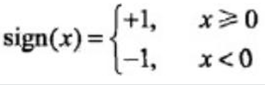
符号函数：

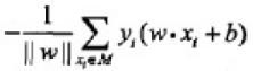
选择误分类点到超平面的总距离作为损失函数：
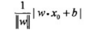
距离：

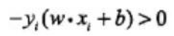
误分类点：

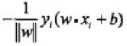
误分类点距离

总距离

感知机对偶形式

过程

例题：


动态可视化代码：

# 以半动画的方式展示感知识机对偶问题的操作的合理性
# 给定初始点， 初始直线
import time

import matplotlib
import numpy as np
from matplotlib.colors import ListedColormap

matplotlib.rcParams['font.sans-serif'] = ['SimHei']
matplotlib.rcParams['font.family']='sans-serif'
matplotlib.rcParams['axes.unicode_minus'] = False
import matplotlib.pyplot as plt


cmap_light = ListedColormap(['#FFAAAA', '#AAFFAA', '#AAAAFF'])
cmap_bold = ListedColormap(['#FF0000', '#00FF00', '#0000FF'])

# 可视化展示
point_coordinates = np.array([2., 2.])  # 关键点坐标

line_a, line_b = 7, 9  # 初始线方程
line_c = - line_b * line_a  # 注意负号

bottom, up = -5, 10  # 视窗

# 关键点对应的“基线”的方程的分类，以平面展示
xx_plane = np.linspace(bottom - 0.5, up + 0.5, 300)
yy_plane = np.linspace(bottom - 0.5, up + 0.5, 300)
xx_plane, yy_plane = np.meshgrid(xx_plane, yy_plane)
class_plane = np.array([1 if np.dot(xi, point_coordinates) + 1 > 0 else 0 for xi in zip(
    xx_plane.ravel(), yy_plane.ravel())]).reshape(xx_plane.shape)

# 优化方程对应的分类，以整数点展示
dots = np.array([np.array([ii, jj]) for ii in range(bottom, up + 1) for jj in range(bottom, up + 1)
                 if ii != point_coordinates[0] or jj != point_coordinates[1]])
class_dots = np.array([1 if np.dot(xi, [line_a, line_b]) + line_c > 0 else 0 for xi in dots])


# 找到直线在视窗内的两个顶点  直线与视窗四线的交点的中间的两个
def window_cross(line_a, line_b, line_c):
    if line_a == 0 and line_b ==0:
        return (0, 0), (0, 0)
    elif line_a == 0:
        return (bottom, -line_c / line_b), (up,  -line_c / line_b)
    elif line_b == 0:
        return (-line_c / line_a, bottom), (-line_c / line_a, up)
    else:
        c1 = bottom, - 1 / line_b * (line_c + line_a * bottom)
        c2 = up, - 1 / line_b * (line_c + line_a * up)
        c3 = -1 / line_a * (line_c + line_b * bottom), bottom
        c4 = -1 / line_a * (line_c + line_b * up), up
        cross_points = [c1, c2, c3, c4]
        cross_points.sort()
        return cross_points[1:3]


# 初始状态展示
plt.figure(figsize=(8, 6))
plt.title('起始状态 同向')
plt.pcolormesh(xx_plane, yy_plane, class_plane, cmap=cmap_light)
plt.scatter(dots[:, 0], dots[:, 1], c=class_dots, cmap=cmap_bold)
color_point = 'b' if point_coordinates[0] * line_a + point_coordinates[1] * line_b + line_c > 0 else 'r'
plt.scatter(point_coordinates[0], point_coordinates[1], c=color_point, marker="v", s=100)
# plt.grid()
plt.plot([bottom - 0.5, up + 0.5], [0, 0], c='k')
plt.plot([0, 0], [bottom - 0.5, up + 0.5], c='k')
cross = window_cross(line_a, line_b, line_c)
plt.plot([cross[0][0], cross[1][0]], [cross[0][1], cross[1][1]], c='g')


# 迭代过程的动态展示
plt.close('all')
plt.figure(figsize=(8, 6))
plt.ion()

for ii in range(200):
    plt.cla()
    plt.title(f'epoch={
      
      ii+1}: ({
      
      line_a}) * x + ({
      
      line_b}) * y + ({
      
      line_c}) = 0', fontsize=20)
    if ii < 8:
        time.sleep(0.4)
    else:
        time.sleep(0.02)
    plt.pcolormesh(xx_plane, yy_plane, class_plane, cmap=cmap_light)
    plt.scatter(dots[:, 0], dots[:, 1], c=class_dots, cmap=cmap_bold)
    color_point = 'b' if point_coordinates[0] * line_a + point_coordinates[1] * line_b + line_c > 0 else 'r'
    plt.scatter(point_coordinates[0], point_coordinates[1], c=color_point, marker="v", s=100)
    plt.grid()
    plt.plot([bottom - 0.5, up + 0.5], [0, 0], c='k')
    plt.plot([0, 0], [bottom - 0.5, up + 0.5], c='k')
    cross = window_cross(line_a, line_b, line_c)
    plt.plot([cross[0][0], cross[1][0]], [cross[0][1], cross[1][1]], c='g')
    # 暂停
    if ii < 8:
        time.sleep(0.3)
    else:
        time.sleep(0.02)
    plt.pause(0.01)
    # 迭代更新
    line_a, line_b, line_c = line_a+point_coordinates[0], line_b+point_coordinates[0], line_c + 1
    class_dots = np.array([1 if np.dot(xi, [line_a, line_b]) + line_c > 0 else 0 for xi in dots])

# 关闭交互模式
plt.ioff()

# 图形显示
plt.show()