深度迁移学习攻略
2.1 应对过拟合
应对过拟合的方法:
(1)增大可以用于训练的数据量
-
数据增强
-
增加数据样本(爬虫、多个数据集、迁移学习-预训练)
(2)让模型能够储存更多地有效信息(量多,但要尽量不相关)
两个:通过控制模型层的数量和层的大小来控制模型中参数的选择;另一种方法是使用权重正则化,如可以使得模型参数值更小的L1或L2正则化。 -
卷积层、池化层、flatten层(后来的网络中用GlobalAveragePooling2D代替了flatten层)
注意卷积核池化的本质就是降维,而由flatten到GlobalAveragePooling2D的变化,从参数的对比可以看出,显然这种改进大大的减少了参数的使用量,避免了过拟合现象。
-
drop out
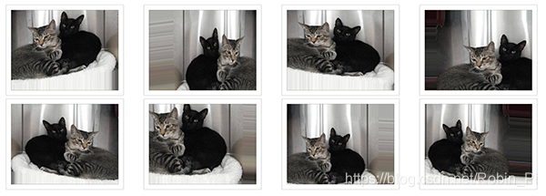
数据增强
Keras ImageDataGenerator and Data Augmentation
from keras.preprocessing.image import ImageDataGenerator

datagen = ImageDataGenerator(
        rotation_range=40,
        width_shift_range=0.2,
        height_shift_range=0.2,
        rescale=1./255,
        shear_range=0.2,
        zoom_range=0.2,
        horizontal_flip=True,
        fill_mode='nearest')
参数理解:
- rotation_range is a value in degrees (0-180), a range within which to randomly rotate pictures
- width_shift and height_shift are ranges (as a fraction of total width or height) within which to randomly translate pictures vertically or horizontally
- rescale is a value by which we will multiply the data before any other processing. Our original images consist in RGB coefficients in the 0-255, but such values would be too high for our models to process (given a typical learning rate), so we target values between 0 and 1 instead by scaling with a 1/255. factor.
- shear_range is for randomly applying shearing transformations
- zoom_range is for randomly zooming inside pictures
- horizontal_flip is for randomly flipping half of the images horizontally --relevant when there are no assumptions of horizontal assymetry (e.g. real-world pictures).
- fill_mode is the strategy used for filling in newly created pixels, which can appear after a rotation or a width/height shift.
例子:
from keras.preprocessing.image import ImageDataGenerator, array_to_img, img_to_array, load_img

datagen = ImageDataGenerator(
        rotation_range=40,
        width_shift_range=0.2,
        height_shift_range=0.2,
        shear_range=0.2,
        zoom_range=0.2,
        horizontal_flip=True,
        fill_mode='nearest')

img = load_img('data/train/cats/cat.0.jpg')  # this is a PIL image
x = img_to_array(img)  # this is a Numpy array with shape (3, 150, 150)
x = x.reshape((1,) + x.shape)  # this is a Numpy array with shape (1, 3, 150, 150)

# the .flow() command below generates batches of randomly transformed images
# and saves the results to the `preview/` directory
i = 0
for batch in datagen.flow(x, batch_size=1,
                          save_to_dir='preview', save_prefix='cat', save_format='jpeg'):
    i += 1
    if i > 20:
        break  # otherwise the generator would loop indefinitely
2.2 评价指标:准确率合适么?
模型验证集准确率的方差很大的的原因会有两方面:一是准确率本身就是一个高方差的评价指;二是用于验证的指标太少。
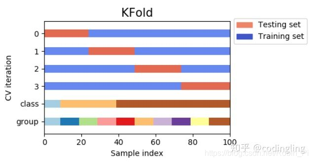
交叉验证
一个好的解决方法就是才用采用交叉验证的方法,比如 k-fold cross-validation,但这也意味着每轮评估需要训练 k 个模型。
# MLP for Pima Indians Dataset with 10-fold cross validation
from keras.models import Sequential
from keras.layers import Dense
from sklearn.model_selection import StratifiedKFold
import numpy
# fix random seed for reproducibility
seed = 7
numpy.random.seed(seed)
# load pima indians dataset
dataset = numpy.loadtxt("pima-indians-diabetes.csv", delimiter=",")
# split into input (X) and output (Y) variables
X = dataset[:,0:8]
Y = dataset[:,8]
# define 10-fold cross validation test harness
kfold = StratifiedKFold(n_splits=10, shuffle=True, random_state=seed)
cvscores = []
for train, test in kfold.split(X, Y):
  # create model
	model = Sequential()
	model.add(Dense(12, input_dim=8, activation='relu'))
	model.add(Dense(8, activation='relu'))
	model.add(Dense(1, activation='sigmoid'))
	# Compile model
	model.compile(loss='binary_crossentropy', optimizer='adam', metrics=['accuracy'])
	# Fit the model
	model.fit(X[train], Y[train], epochs=150, batch_size=10, verbose=0)
	# evaluate the model
	scores = model.evaluate(X[test], Y[test], verbose=0)
	print("%s: %.2f%%" % (model.metrics_names[1], scores[1]*100))
	cvscores.append(scores[1] * 100)
print("%.2f%% (+/- %.2f%%)" % (numpy.mean(cvscores), numpy.std(cvscores)))
一个坑:StratifiedKFold (与 Kfold 不同),它只接受 整数编码
所以,划分时,必须先抓换为整数编码,之后再变回去!
附上:转为独热编码的方法 也可点击
from numpy import array
from numpy import argmax
from sklearn.preprocessing import LabelEncoder
from sklearn.preprocessing import OneHotEncoder
# define example
data = ['cold', 'cold', 'warm', 'cold', 'hot', 'hot', 'warm', 'cold', 'warm', 'hot']
values = array(data)
print(values)
# integer encode
label_encoder = LabelEncoder()
integer_encoded = label_encoder.fit_transform(values)
print(integer_encoded)
# binary encode
onehot_encoder = OneHotEncoder(sparse=False)
integer_encoded = integer_encoded.reshape(len(integer_encoded), 1)
onehot_encoded = onehot_encoder.fit_transform(integer_encoded)
print(onehot_encoded)
# invert first example
inverted = label_encoder.inverse_transform([argmax(onehot_encoded[0, :])])
print(inverted)
Keras 里划分数据集的方法和使用 sklearn 交叉验证集的方法:Keras验证集切分
sk-learn 官方:sklearn之交叉验证

 疑问:
疑问:
random state 设置一个固定值还是?
多维数组的话是按照第一个维度(sample)来进行划分么?
交叉验证和Early stopping如何同时使用?
注意:因为交叉验证没有单独划分验证集,所以没办法用 val_loss 进行监控——monitor 切换为 acc
迁移学习
另一个更加优化的方式是使用在大型数据集上进行预训练了的网络模型。这些模型已经学习到了计算机视觉问题中的绝大数特征,如果直接使用这些特征会让我们获得一个更高的准确率,相比仅使用手头的数据集的话。
(1)微调的两种思路:
(不讨论直接迁移过来,不进行训练直接预测的情况)
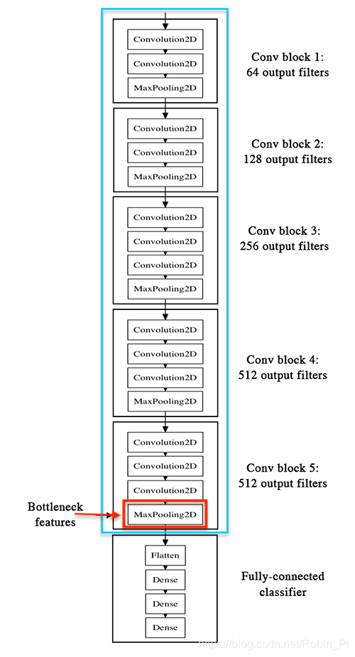
- 使用预训练模型的顶层特征( bottleneck features)——全连接层之前的最后一层的特征图,去训练我们自己的全连接层。
Our strategy will be as follow: we will only instantiate the convolutional part of the model, everything up to the fully-connected layers. We will then run this model on our training and validation data once, recording the output (the “bottleneck features” from th VGG16 model: the last activation maps before the fully-connected layers) in two numpy arrays. Then we will train a small fully-connected model on top of the stored features.
The reason why we are storing the features offline rather than adding our fully-connected model directly on top of a frozen convolutional base and running the whole thing, is computational effiency. Running VGG16 is expensive, especially if you’re working on CPU, and we want to only do it once. Note that this prevents us from using data augmentation.
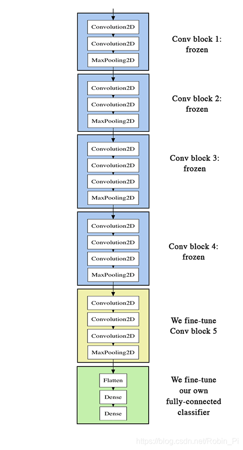
- 微调(Fine-tuning)预训练模型的最后几层( top layers )之后,再利用这些特征去训练我们自己的全连接网络。
注意点:
- in order to perform fine-tuning, all layers should start with properly trained weights: for instance you should not slap a randomly initialized fully-connected network on top of a pre-trained convolutional base. This is because the large gradient updates triggered by the randomly initialized weights would wreck the learned weights in the convolutional base. In our case this is why we first train the top-level classifier, and only then start fine-tuning convolutional weights alongside it.
- we choose to only fine-tune the last convolutional block rather than the entire network in order to prevent overfitting, since the entire network would have a very large entropic capacity and thus a strong tendency to overfit. The features learned by low-level convolutional blocks are more general, less abstract than those found higher-up, so it is sensible to keep the first few blocks fixed (more general features) and only fine-tune the last one (more specialized features).
- fine-tuning should be done with a very slow learning rate, and typically with the SGD optimizer rather than an adaptative learning rate optimizer such as RMSProp. This is to make sure that the magnitude of the updates stays very small, so as not to wreck the previously learned features.
具体以 VGG16 网络为例,使用Keras进行迁移学习:
-
冻结除了全连接层以外的全部的网络,最一层的特征图作为我们训练自己全连接网络的特征。
-
训练全连接之前的最后几层网络,然后将特数据用于自己新定义的网络上进行训练
-
实际代码:以 Fine-tune InceptionV3 为例
from keras.applications.inception_v3 import InceptionV3
from keras.preprocessing import image
from keras.models import Model
from keras.layers import Dense, GlobalAveragePooling2D
from keras import backend as K

# create the base pre-trained model
base_model = InceptionV3(weights='imagenet', include_top=False)

# add a global spatial average pooling layer
x = base_model.output
x = GlobalAveragePooling2D()(x)
# let's add a fully-connected layer
x = Dense(1024, activation='relu')(x)
# and a logistic layer -- let's say we have 200 classes
predictions = Dense(200, activation='softmax')(x)

# this is the model we will train
model = Model(inputs=base_model.input, outputs=predictions)

# first: train only the top layers (which were randomly initialized)
# i.e. freeze all convolutional InceptionV3 layers
for layer in base_model.layers:
    layer.trainable = False

# compile the model (should be done *after* setting layers to non-trainable)
model.compile(optimizer='rmsprop', loss='categorical_crossentropy')

# train the model on the new data for a few epochs
model.fit_generator(...)

# at this point, the top layers are well trained and we can start fine-tuning
# convolutional layers from inception V3. We will freeze the bottom N layers
# and train the remaining top layers.

# let's visualize layer names and layer indices to see how many layers
# we should freeze:
for i, layer in enumerate(base_model.layers):
   print(i, layer.name)

# we chose to train the top 2 inception blocks, i.e. we will freeze
# the first 249 layers and unfreeze the rest:
for layer in model.layers[:249]:
   layer.trainable = False
for layer in model.layers[249:]:
   layer.trainable = True

# we need to recompile the model for these modifications to take effect
# we use SGD with a low learning rate
from keras.optimizers import SGD
model.compile(optimizer=SGD(lr=0.0001, momentum=0.9), loss='categorical_crossentropy')

# we train our model again (this time fine-tuning the top 2 inception blocks
# alongside the top Dense layers
model.fit_generator(...)
等多的关于使用迁移神经网络作为输入特征,或者选取具体某一层的特征图作为特征的方法,可以继续参考 Keras Documentation。
以VGG16为例的迁移学习模板:
# -*- coding: UTF-8 -*-
import keras
from keras import Model
from keras.applications import VGG16
from keras.callbacks import TensorBoard, ModelCheckpoint
from keras.layers import Flatten, Dense, Dropout, GlobalAveragePooling2D
from keras.models import load_model
from keras.preprocessing import image
from PIL import ImageFile
import numpy as np
import tensorflow as tf
from keras.preprocessing.image import ImageDataGenerator
from datetime import datetime
TIMESTAMP = "{0:%Y-%m-%dT%H-%M-%S/}".format(datetime.now())
ImageFile.LOAD_TRUNCATED_IMAGES = True


EPOCHS = 30
BATCH_SIZE = 16
DATA_TRAIN_PATH = 'D:/data/train'


def Train():
    #-------------准备数据--------------------------
    #数据集目录应该是 train/LabelA/1.jpg  train/LabelB/1.jpg这样
    gen = ImageDataGenerator(rescale=1. / 255)
    train_generator = gen.flow_from_directory(DATA_TRAIN_PATH, (224,224)), shuffle=False,
                                              batch_size=BATCH_SIZE, class_mode='categorical')

    #-------------加载VGG模型并且添加自己的层----------------------
    #这里自己添加的层需要不断调整超参数来提升结果,输出类别更改softmax层即可

    #参数说明:inlucde_top:是否包含最上方的Dense层,input_shape:输入的图像大小(width,height,channel)
    base_model = VGG16(weights='imagenet', include_top=False, input_shape=(224, 224, 3))
    x = base_model.output
    x=Flatten()(x)
    x = Dense(256, activation='relu')(x)
    x = Dropout(0.5)(x)
    x = Dense(1, activation='sigmoid')(x)
    predictions = Dense(2, activation='softmax')(x)
    model = Model(input=base_model.input, output=predictions)


    #-----------控制需要FineTune的层数,不FineTune的就直接冻结
    for layer in base_model.layers:
        layer.trainable = False

    #----------编译,设置优化器,损失函数,性能指标
    model.compile(optimizer='rmsprop',
                  loss='binary_crossentropy', metrics=['accuracy'])

    #----------设置tensorboard,用来观察acc和loss的曲线---------------
    tbCallBack = TensorBoard(log_dir='./logs/' + TIMESTAMP,  # log 目录
                             histogram_freq=0,  # 按照何等频率(epoch)来计算直方图,0为不计算
                             batch_size=16,  # 用多大量的数据计算直方图
                             write_graph=True,  # 是否存储网络结构图
                             write_grads=True,  # 是否可视化梯度直方图
                             write_images=True,  # 是否可视化参数
                             embeddings_freq=0,
                             embeddings_layer_names=None,
                             embeddings_metadata=None)

    #---------设置自动保存点,acc最好的时候就会自动保存一次,会覆盖之前的存档---------------
    checkpoint = ModelCheckpoint(filepath='HatNewModel.h5', monitor='acc', mode='auto', save_best_only='True')

    #----------开始训练---------------------------------------------
    model.fit_generator(generator=train_generator,
                        epochs=EPOCHS,
                        callbacks=[tbCallBack,checkpoint],
                        verbose=2
                        )


#-------------预测单个图像--------------------------------------
def Predict(imgPath):
    model = load_model(SAVE_MODEL_NAME)
    img = image.load_img(imgPath, target_size=(224, 224))
    x = image.img_to_array(img)
    x = np.expand_dims(x, axis=0)
    res = model.predict(x)
    print(np.argmax(res, axis=1)[0])
以上运行环境:

Keras2.1.4

Tensorflow-gpu 1.5

CUDA9.0

cudnn7.0

python3.5
更多微调的例例子:
VGG16
VGG19
VGG16 Fine-tuning model
How to make Fine tuning model by Keras
Keras 迁移学习的例子:
Keras预训练模型综合对比
(2)选择那一层的特征作为训练特征的问题
(结合自己之前在CK+上的实验!直接作为结论)
微调前,先查看预训练到的模型:层数和名称:
# check the layers by name
for i,layer in enumerate(vgg_model.layers):
    print(i,layer.name)
2.3 如何提高迁移学习的效果
- 保证测试新的数据集时,也进行跟训练集一样的预处理过程
Edit: To ensure that image is processed in same way as the training
images are processed use keras generator onlysamplewise_std_normalization=True) test_generator = test_datagen.flow_from_directory( args.validate_dir, # this is the target directory target_size=(512, 512), batch_size=batch_size, class_mode='categorical', shuffle=True)Now test_generator.next() will return X,Y pair which can be used for
prediction checks.I have ignored rotations and all from ImageDataGenerator as they are
not changing the image properties like featurewise_center is changing.
模型/特征融合
考虑加融合机器学习分类器学到的特征
Keras Pipeline(custom generator + imgaug)
def create_model(self):
		input_layer = Input(self.input_dim)

		nas_mobile_model = NASNetMobile(include_top=False, input_tensor=input_layer, weights='imagenet')
		x = nas_mobile_model(input_layer)

		# output layers
		x1 = GlobalAveragePooling2D()(x)
		x2 = GlobalMaxPooling2D()(x)
		x3 = Flatten()(x)

		out = Concatenate(axis=-1)([x1, x2, x3])
		out = Dropout(0.5)(out)
		output_layer = Dense(self.n_classes, activation='sigmoid')(out)

		model = Model(inputs=input_layer, outputs=output_layer)

		model.compile(optimizer=Adam(lr=0.0005), loss="binary_crossentropy", metrics=['acc'])
		return model
2.4 输入数据的格式(大小、通道数)
使用深度CNN提取建议区域的特征时,需要注意的是,有些网络对输入图片的大小有要求,如Alex-net要求输入的图片尺寸为227像素*227像素的大小。
全卷网络的输入可以是任意大小,含有全连接层则需固定大小。
(卷积层对于图像是没有尺寸限制要求)——需要好好研究
模型数据格式(大小、通道数)的限制问题:默认要求输入彩色图和一定大小 (224x224)
(1)例如通道数的问题:
(三通道) 预训练数据应用到(单通道)灰度图,可能出现的问题:
- 数据格式不对——只能强制性转换数据:
① 一维到三维(repeat 一维灰度图到3维)
faces = np.repeat(faces, 3, -1)
② 三维到一维(只提出一维卷积数据 or 将特征图flaten到一维)
img_input = Input(shape=(img_size_target,img_size_target,1))
img_conc = Concatenate()([img_input, img_input, img_input])

model = Unet(backbone_name='resnet34', input_tensor=img_conc, encoder_weights='imagenet', freeze_encoder=True)
(2)又或者迁移神经网络对输入数据有最小尺寸的要求,比如VGG16,最小为48x48——用opencv转换是否合算?
DeepLearning(keras框架)–图像输入大小及通道调整问题
——直接改变迁移网络的输入input?(因为)
# load model without classifier layers
model = VGG16(include_top=False, input_shape=(48, 48, 3))
值得注意的是,如果输入大小不是224也不要紧,只要在全连接层之前使用全局平均池化就行。(但是需要满足预训练网络的最小尺寸大小,比如VGG16最小尺寸是48x48 查看)
If your model uses a global average pooling before the “dense” classification layer, then it does not matter how large the inputs are. You can input a 600x480 image and the model will give a prediction for the full image.
However, if you wanted to take 224x224 crops from the 600x480 image, you could first resize it so the smallest side is 256. That would make the input image 320x256. Now you can take 224x224 crops from this resized image.
模型小型化(降维)
(类似从VGG到Inception的操作)
Commonly used CNNs for feature extraction include a set of fully connected layers at the end. Fully connected layers tend to contain most of the parameters in a CNN. Specifically, VGG16 [10] contains approximately 90% of all its parameters in their last fully connected layers. Recent architectures such as Inception V3 [12], reduced the amount of parameters in their last layers by including a Global Average Pooling operation. Global Average Pooling reduces each feature map into a scalar value by taking the average over all elements in the feature map. The average operation forces the network to extract global features from the input image. Modern CNN architectures such as Xception [1] leverage from the combination of two of the most successful experimental assumptions in CNNs: the use of residual modules [6] and depth-wise separable convolutions [2]. Depth-wise separable convolutions reduce further the amount of parameters by separating the processes of feature extraction and combination within a convolutional layer.
如何手动打乱多维数据
打乱 多维的 X
-
打乱第一个轴:np.random.shuffle(arr)
This function only shuffles the array along the first axis of a multi-dimensional array. The order of sub-arrays is changed but
their contents remains the same.Parameter
---------- x : array_like
The array or list to be shuffled.Returns
------- None -
打乱指定的轴 :apply_along_axis
import numpy as np
a = np.arange(40).reshape((5,8))
# shuffle along axis 1
np.apply_along_axis(np.random.shuffle,1,a)
shuffle along axis 0
np.random.shuffle(a)
print(a)
打乱多维的 X 和 y
只需对下面代码进行些许修改,将 len(data) 换为第一维 大小
# 随机打乱 序列
index = [i for i in range(len(data))]
random.shuffle(index)
data = data[index]
label = label[index]
结果如下:
# 随机打乱多维数组 X 和 y (三维数据)
import random
X = np.arange(0, 12).reshape(2, 3, 2)

Y = np.arange(0, 10, 6).reshape(-1, 1)
print(X)
print(Y)
index = [i for i in range(X.shape[0])]
# print(index)
random.shuffle(index)

X = X[index]
Y = Y[index]

# print(X.shape, Y.shape)
print(X)
print(Y)
[[[ 0  1]
  [ 2  3]
  [ 4  5]]

 [[ 6  7]
  [ 8  9]
  [10 11]]]
[[0]
 [6]]
[[[ 6  7]
  [ 8  9]
  [10 11]]

 [[ 0  1]
  [ 2  3]
  [ 4  5]]]
[[6]
 [0]]
# 随机打乱多维数组 X 和 y  (四维数据)
import random
X = np.arange(0, 16).reshape(2, 2, 2, 2)

Y = np.arange(0, 2).reshape(-1, 1)
print(X)
print(Y)
index = [i for i in range(X.shape[0])]
# print(index)
random.shuffle(index)

X = X[index]
Y = Y[index]

print(X.shape, Y.shape)
print(X)
print(Y)
[[[[ 0  1]
   [ 2  3]]

  [[ 4  5]
   [ 6  7]]]


 [[[ 8  9]
   [10 11]]

  [[12 13]
   [14 15]]]]
[[0]
 [1]]
(2, 2, 2, 2) (2, 1)
[[[[ 8  9]
   [10 11]]

  [[12 13]
   [14 15]]]


 [[[ 0  1]
   [ 2  3]]

  [[ 4  5]
   [ 6  7]]]]
[[1]
 [0]]
2.4 模型训练
如何划分:训练集、验证集和测试集
比较全面的经验:深度学习Keras采坑经验
2.5 分析与可视化
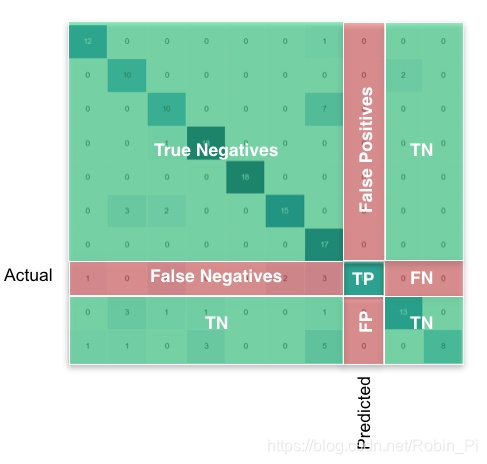
混淆矩阵
-
需要注意的是:
y_test 需要由 one-hot 编码格式变为 个位数字代表的编码。
不然会出现如下报错:
confusion matrix error “Classification metrics can’t handle a mix of multilabel-indicator and multiclass targets” -
解决:
import numpy as np
rounded_labels=np.argmax(test_labels, axis=1)
rounded_labels[1]
1 .python实现混淆矩阵
2. 数据可视化-混淆矩阵(confusion matrix)
- 最简例子1:
# 混淆矩阵

import seaborn as sns
from sklearn.metrics import confusion_matrix
import matplotlib.pyplot as plt

sns.set()
f,ax=plt.subplots()
y_true = [0,0,1,2,1,2,0,2,2,0,1,1]
y_pred = [1,0,1,2,1,0,0,2,2,0,1,1]
C2= confusion_matrix(y_true, y_pred, labels=[0, 1, 2])
print(C2) #打印出来看看
sns.heatmap(C2,annot=True,ax=ax) #画热力图

ax.set_title('Confusion matrix') #标题
ax.set_xlabel('Predict') #x轴
ax.set_ylabel('True') #y轴
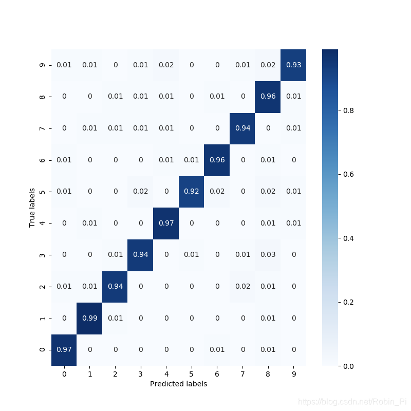
- 例子2:
import keras
import matplotlib.pyplot as plt
import numpy as np
import seaborn as sns

from sklearn.metrics import confusion_matrix

# === dataset ===
with np.load('mnist.npz') as f:
    x_train, y_train = f['x_train'], f['y_train']
    x_test, y_test = f['x_test'], f['y_test']

x_train = x_train.reshape(60000, 28, 28, 1)
x_test = x_test.reshape(10000, 28, 28, 1)
print(x_train.shape)
print(x_test.shape)

# === model: CNN ===
model = keras.models.Sequential()
model.add(keras.layers.Conv2D(32, (3, 3), activation='relu', input_shape=(28, 28, 1)))
model.add(keras.layers.MaxPooling2D((2, 2)))
model.add(keras.layers.Conv2D(64, (3, 3), activation='relu'))
model.add(keras.layers.MaxPooling2D((2, 2)))
model.add(keras.layers.Flatten())
model.add(keras.layers.Dense(64, activation='relu'))
model.add(keras.layers.Dense(10, activation='softmax'))
model.compile(optimizer='adam',
              loss='sparse_categorical_crossentropy',
              metrics=['accuracy'])
model.summary()

# === train ===
model.fit(x=x_train, y=y_train,
          batch_size=512,
          epochs=10,
          validation_data=(x_test, y_test))

# === pred ===
y_pred = model.predict_classes(x_test)
print(y_pred)

# === 混淆矩阵:真实值与预测值的对比 ===
# https://scikit-learn.org/stable/auto_examples/model_selection/plot_confusion_matrix.html
con_mat = confusion_matrix(y_test, y_pred)

con_mat_norm = con_mat.astype('float') / con_mat.sum(axis=1)[:, np.newaxis]     # 归一化
con_mat_norm = np.around(con_mat_norm, decimals=2)

# === plot ===
plt.figure(figsize=(8, 8))
sns.heatmap(con_mat_norm, annot=True, cmap='Blues')

plt.ylim(0, 10)
plt.xlabel('Predicted labels')
plt.ylabel('True labels')
plt.show()
如何调整学习率、如何实现“早停”
比较全面的经验:深度学习Keras采坑经验
模型的可视化
这部分:更详细
Keras Documentation-Model visualization
from keras.applications.vgg16 import VGG16
from keras.utils.vis_utils import plot_model
model = VGG16()
plot_model(model, to_file='vgg.png')
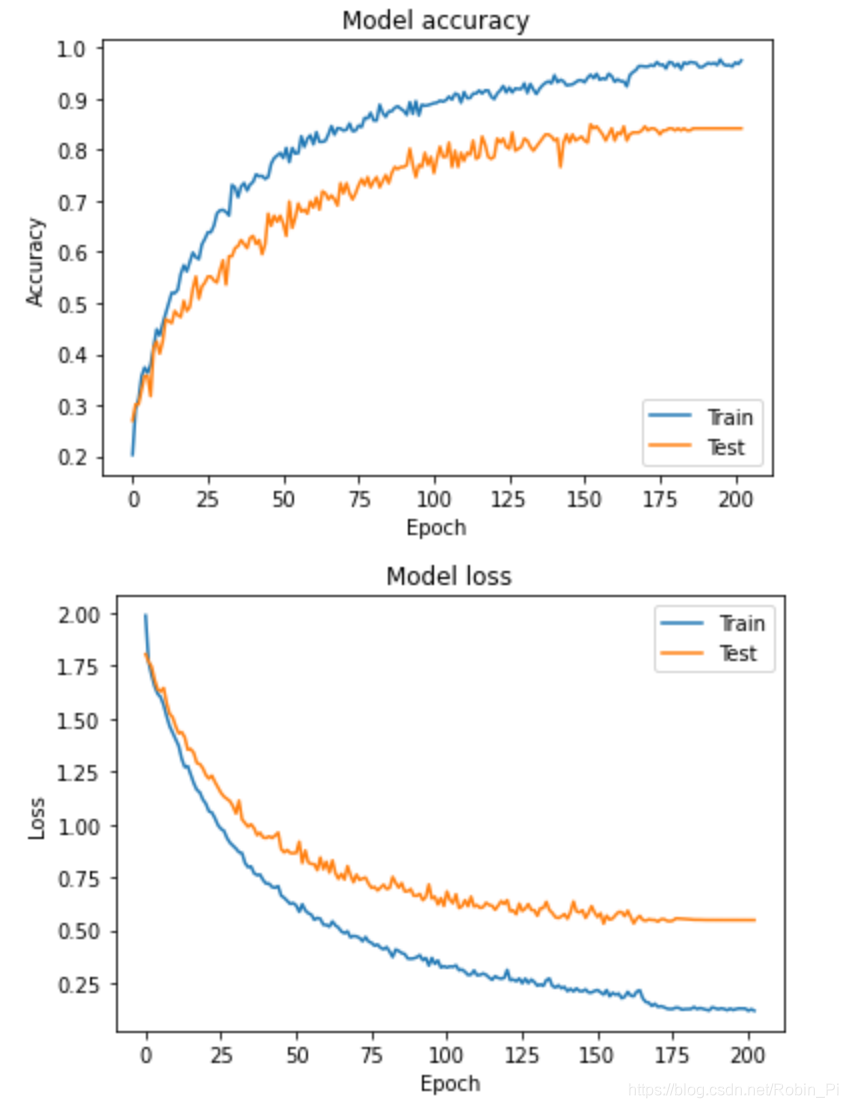
训练过程可视化
(1)方法一:
import matplotlib.pyplot as plt

history = model.fit(x, y, validation_split=0.25, epochs=50, batch_size=16, verbose=1)

# Plot training & validation accuracy values
plt.plot(history.history['acc'])
plt.plot(history.history['val_acc'])
plt.title('Model accuracy')
plt.ylabel('Accuracy')
plt.xlabel('Epoch')
plt.legend(['Train', 'Test'], loc='upper left')
plt.show()

# Plot training & validation loss values
plt.plot(history.history['loss'])
plt.plot(history.history['val_loss'])
plt.title('Model loss')
plt.ylabel('Loss')
plt.xlabel('Epoch')
plt.legend(['Train', 'Test'], loc='upper left')
plt.show()
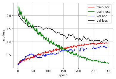
(2)方法二
import keras

#写一个LossHistory类,保存loss和acc
class LossHistory(keras.callbacks.Callback):
    def on_train_begin(self, logs={

    }):
        self.losses = {

    'batch': [], 'epoch': []}
        self.accuracy = {

    'batch': [], 'epoch': []}
        self.val_loss = {

    'batch': [], 'epoch': []}
        self.val_acc = {

    'batch': [], 'epoch': []}

    def on_batch_end(self, batch, logs={

    }):
        self.losses['batch'].append(logs.get('loss'))
        self.accuracy['batch'].append(logs.get('acc'))
        self.val_loss['batch'].append(logs.get('val_loss'))
        self.val_acc['batch'].append(logs.get('val_acc'))

    def on_epoch_end(self, batch, logs={

    }):
        self.losses['epoch'].append(logs.get('loss'))
        self.accuracy['epoch'].append(logs.get('acc'))
        self.val_loss['epoch'].append(logs.get('val_loss'))
        self.val_acc['epoch'].append(logs.get('val_acc'))

    def loss_plot(self, loss_type):
        iters = range(len(self.losses[loss_type]))
        #创建一个图
        plt.figure()
        # acc
        plt.plot(iters, self.accuracy[loss_type], 'r', label='train acc')#plt.plot(x,y),这个将数据画成曲线
        # loss
        plt.plot(iters, self.losses[loss_type], 'g', label='train loss')
        if loss_type == 'epoch':
            # val_acc
            plt.plot(iters, self.val_acc[loss_type], 'b', label='val acc')
            # val_loss
            plt.plot(iters, self.val_loss[loss_type], 'k', label='val loss')
        plt.grid(True)#设置网格形式
        plt.xlabel(loss_type)
        plt.ylabel('acc-loss')#给x,y轴加注释
        plt.legend(loc="upper right")#设置图例显示位置
        plt.show()

# 创建一个实例history
history = LossHistory()
再其放入 fit 函数 callbacks=[history]) #callbacks回调,将数据传给history
特征图/模型可视化
CNN 卷积核/层输出可视化
- Keras实现卷积神经网络(CNN)可视化
- 可视化卷积核 Visualizing convnet filters
- keras CNN卷积核可视化,热度图
- keras训练曲线,混淆矩阵,CNN层输出可视化
- 使用神经网络可视化 去看网络中间层提取的特征
模型保存
Callback 回调是Keras的一个类,是在训练过程的特定阶段调用的一组函数,可以使用回调来获取训练期间内部状态和模型统计信息的视图。
Callback 方法:
-
History
History对象即为fit方法的返回值 -
ModelCheckpoint
该回调函数将在每个epoch后保存模型到filepath -
TensorBoard
该回调函数是一个可视化的展示器 -
CSVLogger
将epoch的训练结果保存在csv文件中,支持所有可被转换为string的值,包括1D的可迭代数值如np.ndarray. -
LambdaCallback
用于创建简单的callback的callback类
训练过程为什么震荡?——试着增大 batch size
训练过程曲线分析:acc/loss/val_acc/val_loss
如设置神经网络参数
bath_size
学习率
卷积核的的大小、卷积步长和卷积核的个数
-
卷积核的的大小
卷积核大小(Kernel Size)
定义了卷积操作的感受野(Receptive Field)。在二维卷积中,通常设置为 3 ,即卷积核大小为 3×3。
卷积核大小,一般都是 奇数x奇数 。直观的理解是,奇数形态的卷积核有中心点,对边沿、对线条更加敏感,可以更有效的提取边沿信息。如果是偶数的话,效率会相对较差,积累起来整体效率就会非常差。
卷积核的大小越大,其感受野(Receptive Field)越大,看到的信息越多,提取的特征就会越优秀。
但是尺寸越大,其计算量就越大,对于有限算力而言,因其训练时间过长,不利于训练模型,也不利于加深网络。 -
步长
步幅(Stride)
定义了卷积核遍历图像时的步幅大小。其默认值通常设置为 1 ,也可将步幅设置为 2 后对图像进行下采样,这种方式与最大池化类似。
…
小结:
一个卷积核的尺寸越大,其感受野越大,所能提取的特征就越优异,但是其参数量也会几何倍数地增长,在现有算力的情况下,不利于网络训练及加深。
为了更快的训练网络并加深网络,我们要找一种「减少参数量,但不影响精度」的解决办法。于是产生了:
- 利用多个小卷积核替代一个大的卷积核(减少参数量)
- 先使用 1x1 卷积核将输入数据降维的 Bottleneck 技术(减少参数量)
- 相当于 5x5 卷积核的 3x3 空洞卷积核 [扩张率为 1 ](减少参数量)
- 单一尺寸卷积核用多尺寸卷积核代替(多尺度观察)
- 参数量不变(3x3),但是提取有效信息更多的 可变形卷积核
综合经验
-
A practical theory for designing very deep convolutional neural networks
实践(从零开始不断的trial-and-error)
Using convolutional neural nets to detect facial keypoints tutorial
参考:
博客
- Keras Documentation
- Illustrated: 10 CNN Architectures
- keras系列︱迁移学习:利用InceptionV3进行fine-tuning及预测、完美案例(五)
- 深度学习在表情识别中的应用
- Building powerful image classification models using very little data
- DeepLearning(keras框架)–图像输入大小及通道调整问题
- Display Deep Learning Model Training History in Keras
论文