py-MDNet详解附代码（二）:online tracking

Overall procedure
Initial test frame
- training
- BBox regression
Subsequent frames update
Hard negative mining
Results on OTB100
Demo
Bonus
References

关于训练部分，可以看上一篇博客： py-MDNet代码提炼(一):train
这篇主要讲解tracking的部分，内容会比训练阶段要复杂一些。
如果不看论文的在线跟踪部分，或者只看了上一篇博客，那不禁就会有很多问题，下面以 问答的形式点出几个要点：
问答形式的开题

Overall procedure

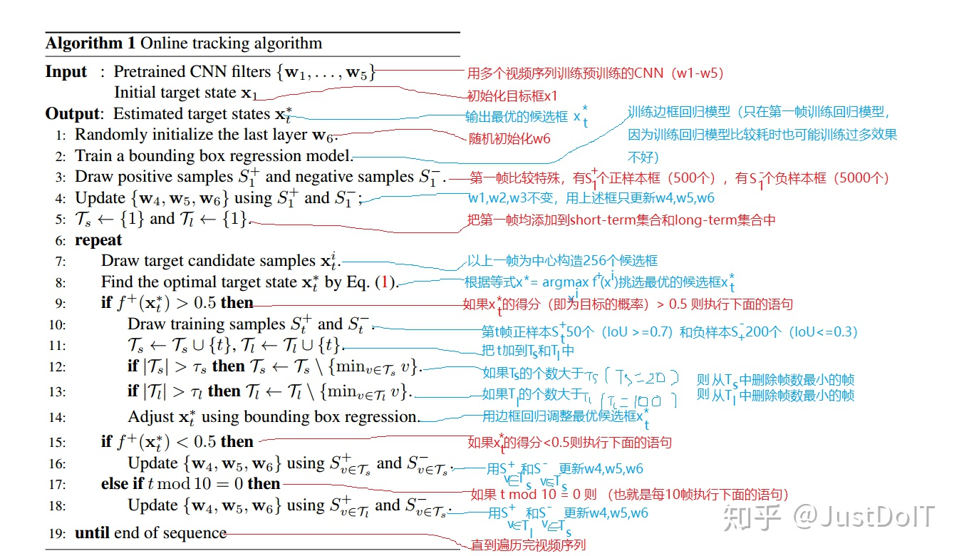
其实tracking阶段主要就是要做上图绿色的四点，整体的过程就如论文中描写的：

输入：训练好的网络模型和第一帧目标状态
输出：后续帧的预测的目标状态

下面就按照整个流程来说明这四点：

Initial test frame

training

在加载完 $w_{1}-w{5}$ 完后，会冻结conv1,conv2,conv3,在训练阶段更新全连接层和新的domain-specific layer，如论文中说的：

the multiple branches of domain-specific layers ( $fc6^{1}$ - $fc6^{K}$ ) are replaced with a single branch (fc6) for a new test sequence. Then we fine-tune the new domain-specific layer and the fully connected layers in the shared network online at the same time

就是上面【line3-4】说的，用 $S_{1}^{+}=500$ 个positive samples和 $S_{1}^{-}=5000$ 个negative samples去训练网络，更新网络的 $w_{3},w_{4},w_{5}$ ，这在代码中就是run_tracker.py中的：

# Draw pos/neg samples
pos_examples = SampleGenerator('gaussian', image.size, opts['trans_pos'], opts['scale_pos'])(
                    target_bbox, opts['n_pos_init'], opts['overlap_pos_init'])
# 500
neg_examples = np.concatenate([
                SampleGenerator('uniform', image.size, opts['trans_neg_init'], opts['scale_neg_init'])(
                    target_bbox, int(opts['n_neg_init'] * 0.5), opts['overlap_neg_init']),
                SampleGenerator('whole', image.size)(
                    target_bbox, int(opts['n_neg_init'] * 0.5), opts['overlap_neg_init'])])
neg_examples = np.random.permutation(neg_examples)
# 5000
# Extract pos/neg features
pos_feats = forward_samples(model, image, pos_examples)
neg_feats = forward_samples(model, image, neg_examples)

# Initial training including hard negative mining
train(model, criterion, init_optimizer, pos_feats, neg_feats, opts['maxiter_init'])
del init_optimizer, neg_feats
torch.cuda.empty_cache()

BBox regression

这也是在第一帧的时候做的，做bounding box regression是为了improve target localization accuracy,因为随机生成的candidates并不一定是很贴合目标的：

we train a simple linear regression model to predict the precise target location using conv3 features of the samples near the target location.
For bounding-box regression, we use 1000 training examples with the same parameters as [13]

这里就是调用from sklearn.linear_model import Ridge来建立线性模型，具体可看下面这幅图：
bbox regression图示

当然只有在success需要进行包围框的回归，论文中是：

In the subsequent frames, we adjust the target locations estimated from Eq. (1) using the regression model if the estimated targets are reliable (i.e. $f^{+}(x^{*})$ > 0.5).

这里判断为reliable的条件可能与论文并不一样，而是通过pos_score的前5名的均值是否大于0来判断，大于0则认为success，代码中是这样体现的：

# Train bbox regressor
bbreg_examples = SampleGenerator('uniform', image.size, opts['trans_bbreg'], opts['scale_bbreg'], opts['aspect_bbreg'])(
    target_bbox, opts['n_bbreg'], opts['overlap_bbreg'])
bbreg_feats = forward_samples(model, image, bbreg_examples)
bbreg = BBRegressor(image.size)
bbreg.train(bbreg_feats, bbreg_examples, target_bbox)
# bbreg_feats [1000, 512*3*3]
# bbreg_examples [1000, 4]
# target_bbox [4,]
########### 使用的时候使用predict方法 #########
bbreg_samples = samples[top_idx]
if top_idx.shape[0] == 1:
    bbreg_samples = bbreg_samples[None,:]
bbreg_feats = forward_samples(model, image, bbreg_samples)
bbreg_samples = bbreg.predict(bbreg_feats, bbreg_samples)
bbreg_bbox = bbreg_samples.mean(axis=0)

Subsequent frames update

在利用第一帧的先验信息后，就得循环预测序列中的后续帧中的目标状态，也就是上面【line6-18】在做的。
首先在上一帧预测的target location构造265个candidates,然后送入网络得到得分，然后挑选pos_score最高的5个candidates，平均他们的位置作为预测出来的target bbox，然后这时会分两种情况：

success:
- 1、进行bounding-box regression
- 2、把此时预测出来的target bbox周围的 $S_{t}^{+}=50$ 个positive samples和 $S_{t}^{-}=200$ 个negative samples的特征并入short-term特征集合 $\mathcal{T}_{s}$ 和long-term特征集合 $\mathcal{T}_{l}$ 中，以备后续更新模型时使用（如果超出规定集合元素上限，则删去最前面的特征）
not success:
- 1、扩大搜索区域（通过扩大samples中心的偏移距离来实现）
- 2、用short-term的特征集合中的特征 $S_{v \in \mathcal{T}_{s}}^{+}$ and $S_{v \in \mathcal{T}_{s}}^{-}$ 来更新模型，来solve target appearance change
经过10帧就进行一次long-term update(这里之所以称作long-term update,是因为使用了long-term features $S_{v \in \mathcal{T}_{l}}^{+}$ 和 $S_{v \in \mathcal{T}_{s}}^{-}$ )

代码中的体现：

# Bbox regression
if success:
    bbreg_samples = samples[top_idx]
    if top_idx.shape[0] == 1:
        bbreg_samples = bbreg_samples[None,:]
    bbreg_feats = forward_samples(model, image, bbreg_samples)
    bbreg_samples = bbreg.predict(bbreg_feats, bbreg_samples)
    bbreg_bbox = bbreg_samples.mean(axis=0)
else:
    bbreg_bbox = target_bbox
    

# Data collect
if success:
    pos_examples = pos_generator(target_bbox, opts['n_pos_update'], opts['overlap_pos_update'])
    pos_feats = forward_samples(model, image, pos_examples)
    pos_feats_all.append(pos_feats)
    if len(pos_feats_all) > opts['n_frames_long']:
        del pos_feats_all[0]

    neg_examples = neg_generator(target_bbox, opts['n_neg_update'], opts['overlap_neg_update'])
    neg_feats = forward_samples(model, image, neg_examples)
    neg_feats_all.append(neg_feats)
    if len(neg_feats_all) > opts['n_frames_short']:
        del neg_feats_all[0]

# Expand search area at failure
if success:
    sample_generator.set_trans(opts['trans'])
else:
    sample_generator.expand_trans(opts['trans_limit'])
    
# Short term update
if not success:
    nframes = min(opts['n_frames_short'], len(pos_feats_all))
    pos_data = torch.cat(pos_feats_all[-nframes:], 0)
    neg_data = torch.cat(neg_feats_all, 0)
    train(model, criterion, update_optimizer, pos_data, neg_data, opts['maxiter_update'])

# Long term update
elif i % opts['long_interval'] == 0:
    pos_data = torch.cat(pos_feats_all, 0)
    neg_data = torch.cat(neg_feats_all, 0)
    train(model, criterion, update_optimizer, pos_data, neg_data, opts['maxiter_update'])

Hard negative mining

难例挖掘就是为了一些困难负样本用来训练分类器，使得对相似物体具有更强的分辨力，难例挖掘是在用初始帧进行初始训练的时候进行的，从1024个negative samples中选择96个pos_score最高的negative samples来作为难例负样本送入分类器的训练。下面是我训练过程中的可视化：
在这里插入图片描述