4.1模型构造
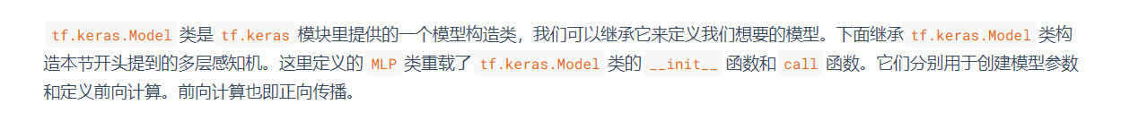
class MLP(tf.keras.Model):
    def __init__(self):
        super().__init__()
        self.flatten = tf.keras.layers.Flatten()    # Flatten层将除第一维(batch_size)以外的维度展平
        self.dense1 = tf.keras.layers.Dense(units=256, activation=tf.nn.relu)
        self.dense2 = tf.keras.layers.Dense(units=10)

    def call(self, inputs):
        x = self.flatten(inputs)
        x = self.dense1(x)
        output = self.dense2(x)
        return output
X = tf.random.uniform((2,20))
net = MLP()
net(X)
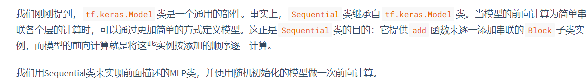
model = tf.keras.models.Sequential([
    tf.keras.layers.Flatten(),
    tf.keras.layers.Dense(256, activation=tf.nn.relu),
    tf.keras.layers.Dense(10),
])

model(X)

class FancyMLP(tf.keras.Model):
    def __init__(self):
        super().__init__()
        self.flatten = tf.keras.layers.Flatten()
        self.rand_weight = tf.constant(
            tf.random.uniform((20,20)))
        self.dense = tf.keras.layers.Dense(units=20, activation=tf.nn.relu)

    def call(self, inputs):
        x = self.flatten(inputs)
        x = tf.nn.relu(tf.matmul(x, self.rand_weight) + 1)
        x = self.dense(x)
        while tf.norm(x) > 1:
            x /= 2
        if tf.norm(x) < 0.8:
            x *= 10
        return tf.reduce_sum(x)

class NestMLP(tf.keras.Model):
    def __init__(self):
        super().__init__()
        self.net = tf.keras.Sequential()
        self.net.add(tf.keras.layers.Flatten())
        self.net.add(tf.keras.layers.Dense(64, activation=tf.nn.relu))
        self.net.add(tf.keras.layers.Dense(32, activation=tf.nn.relu))
        self.dense = tf.keras.layers.Dense(units=16, activation=tf.nn.relu)


    def call(self, inputs):
        return self.dense(self.net(inputs))

net = tf.keras.Sequential()
net.add(NestMLP())##########直接利用函数add
net.add(tf.keras.layers.Dense(20))
net.add(FancyMLP())#######

net(X)
4.2模型参数的访问、初始化和共享
net = tf.keras.models.Sequential()
net.add(tf.keras.layers.Flatten())
net.add(tf.keras.layers.Dense(256,activation=tf.nn.relu))
net.add(tf.keras.layers.Dense(10))

X = tf.random.uniform((2,20))
Y = net(X)
Y
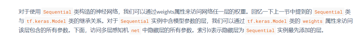
net.weights[0], type(net.weights[0])
(<tf.Variable 'sequential/dense/kernel:0' shape=(20, 256) dtype=float32, numpy=
 array([[-0.07852519, -0.03260126,  0.12601742, ...,  0.11949158,
          0.10042094, -0.10598273],
        [ 0.03567271, -0.11624913,  0.04699135, ..., -0.12115637,
          0.07733515,  0.13183317],
        [ 0.03837337, -0.11566538, -0.03314627, ..., -0.10877015,
          0.09273799, -0.07031895],
        ...,
        [-0.03430544, -0.00946991, -0.02949082, ..., -0.0956497 ,
         -0.13907745,  0.10703176],
        [ 0.00447187, -0.07251608,  0.08081181, ...,  0.02697623,
          0.05394638, -0.01623751],
        [-0.01946831, -0.00950103, -0.14190955, ..., -0.09374787,
          0.08714674,  0.12475103]], dtype=float32)>,
 tensorflow.python.ops.resource_variable_ops.ResourceVariable)

class Linear(tf.keras.Model):
    def __init__(self):
        super().__init__()
        self.d1 = tf.keras.layers.Dense(
            units=10,
            activation=None,
            kernel_initializer=tf.random_normal_initializer(mean=0,stddev=0.01),
            bias_initializer=tf.zeros_initializer()
        )
        self.d2 = tf.keras.layers.Dense(
            units=1,
            activation=None,
            kernel_initializer=tf.ones_initializer(),
            bias_initializer=tf.ones_initializer()
        )

    def call(self, input):
        output = self.d1(input)
        output = self.d2(output)
        return output

net = Linear()
net(X)
net.get_weights()
[array([[-0.00306494,  0.01149799,  0.00900665, -0.00952527, -0.00651997,
      0.00010531,  0.00802666, -0.01102469,  0.01838934,  0.00915548],
    [ 0.00401672,  0.01788972, -0.00245794, -0.01051202,  0.02268461,
     -0.00271502, -0.00447782,  0.00636486,  0.00408998, -0.01373187],
    [-0.00468962, -0.00180526, -0.0117501 ,  0.01840584,  0.00044537,
     -0.00745311,  0.01155732, -0.00615015, -0.00942082, -0.00023081],
    [-0.01116156, -0.00614527, -0.00119119, -0.00843481,  0.01192368,
      0.00889105, -0.01000126, -0.0017869 , -0.00833272,  0.0019026 ],
    [ 0.0183291 , -0.00640716,  0.00936602,  0.01040828, -0.00140882,
     -0.00143817,  0.00126366,  0.01094474,  0.0132029 ,  0.00405393],
    [-0.00548183, -0.00489746, -0.01264372, -0.00501967,  0.00602909,
      0.00439432,  0.02449438,  0.00426046, -0.0017243 , -0.00319188],
    [-0.00034199, -0.00648715, -0.00694025, -0.00984227,  0.02798587,
     -0.01283635, -0.01735584, -0.00181439,  0.01585936,  0.00348289],
    [ 0.00181157, -0.00343991,  0.01415697, -0.00160312,  0.0018713 ,
     -0.00968461, -0.00268579,  0.01320006, -0.00041133, -0.01282531],
    [-0.0145638 ,  0.0096653 , -0.00787722, -0.00073892, -0.00222261,
      0.0031008 , -0.01858314,  0.00559973,  0.00439452, -0.02467434],
    [-0.00303086,  0.0015006 , -0.00920389,  0.01035136, -0.00040001,
     -0.00945453, -0.00506378,  0.00816534,  0.00347233,  0.01201165],
    [ 0.01979353,  0.00881971, -0.00060045, -0.00671935,  0.02482731,
     -0.0039808 ,  0.01195751, -0.00499541, -0.01421177,  0.00125722],
    [-0.00206965,  0.00737946,  0.02711954, -0.00566722, -0.01916223,
      0.00635906, -0.00112362,  0.00351852,  0.0027598 ,  0.00804986],
    [ 0.00190901,  0.00799948, -0.01007551, -0.00751526,  0.0027352 ,
     -0.00126002,  0.00079498, -0.00190032, -0.00912007,  0.00432031],
    [-0.00574654,  0.00703932,  0.00375365,  0.01700558, -0.00392553,
      0.00246399,  0.00686003, -0.00327425, -0.00158563,  0.01139532],
    [-0.010441  , -0.01566261,  0.01807244, -0.01265192, -0.00422926,
     -0.00729915, -0.00717674, -0.00036729,  0.00728995,  0.0034066 ],
    [-0.00497032, -0.01395558, -0.00276683,  0.0114197 , -0.01044411,
     -0.01518542,  0.00793149, -0.00169621, -0.008745  , -0.00825851],
    [-0.00098009, -0.00765272, -0.01993775,  0.0207908 , -0.0088134 ,
      0.01211826,  0.0033179 ,  0.0064116 ,  0.00399073,  0.00067746],
    [ 0.00282402,  0.00589997,  0.00674444, -0.01209166, -0.00875635,
      0.01789016, -0.00037993,  0.00392861,  0.02248183, -0.00427692],
    [-0.00629026, -0.01388059,  0.0160582 ,  0.00855581,  0.00170209,
      0.00430258,  0.0092911 ,  0.00232163,  0.00591121,  0.02038265],
    [-0.00792203, -0.00259904, -0.00109487, -0.00959524, -0.00030968,
     -0.01322429,  0.00489308,  0.00503101,  0.01801165,  0.00972504]],
   dtype=float32),
 array([0., 0., 0., 0., 0., 0., 0., 0., 0., 0.], dtype=float32),
 array([[1.],
        [1.],
        [1.],
        [1.],
        [1.],
        [1.],
        [1.],
        [1.],
        [1.],
        [1.]], dtype=float32),
 array([1.], dtype=float32)]
可以使用tf.keras.initializers类中的方法实现自定义初始化。
def my_init():
    return tf.keras.initializers.Ones()

model = tf.keras.models.Sequential()
model.add(tf.keras.layers.Dense(64, kernel_initializer=my_init()))

Y = model(X)
model.weights[0]
<tf.Variable 'sequential_1/dense_4/kernel:0' shape=(20, 64) dtype=float32, numpy=
array([[1., 1., 1., ..., 1., 1., 1.],
       [1., 1., 1., ..., 1., 1., 1.],
       [1., 1., 1., ..., 1., 1., 1.],
       ...,
       [1., 1., 1., ..., 1., 1., 1.],
       [1., 1., 1., ..., 1., 1., 1.],
       [1., 1., 1., ..., 1., 1., 1.]], dtype=float32)>
4.3模型参数的延后初始化
TF2.0版本 404 了,因此参考了 pytoch 版本
https://www.bookstack.cn/read/d2l-ai-d2l-zh/408bd3f458c80a63.md
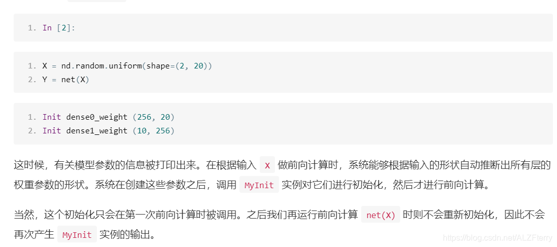
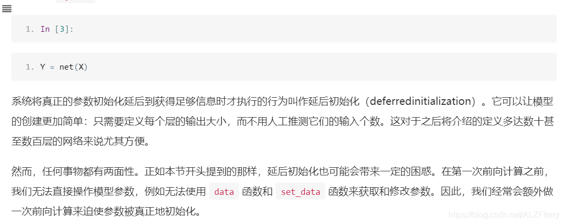
也许读者早就注意到了,在之前使用Gluon创建的全连接层都没有指定输入个数。例如,在上一节使用的多层感知机net里,我们创建的隐藏层仅仅指定了输出大小为256。当调用initialize函数时,由于隐藏层输入个数依然未知,系统也无法得知该层权重参数的形状。只有在当我们将形状是(2,20)的输入X传进网络做前向计算net(X)时,系统才推断出该层的权重参数形状为(256,20)。因此,这时候我们才能真正开始初始化参数。
让我们使用上一节中定义的MyInit类来演示这一过程。我们创建多层感知机,并使用MyInit实例来初始化模型参数。
from mxnet import init, nd
from mxnet.gluon import nn

class MyInit(init.Initializer):
    def _init_weight(self, name, data):
        print('Init', name, data.shape)
        # 实际的初始化逻辑在此省略了

net = nn.Sequential()
net.add(nn.Dense(256, activation='relu'),
        nn.Dense(10))

net.initialize(init=MyInit())
注意,虽然MyInit被调用时会打印模型参数的相关信息,但上面的initialize函数执行完并未打印任何信息。由此可见,调用initialize函数时并没有真正初始化参数。下面我们定义输入并执行一次前向计算。
4.4自定义层
我们先介绍如何定义一个不含模型参数的自定义层。事实上,这和[“模型构造”]一节中介绍的使用tf.keras.Model类构造模型类似。下面的CenteredLayer类通过继承tf.keras.layers.Layer类自定义了一个将输入减掉均值后输出的层,并将层的计算定义在了call函数里。这个层里不含模型参数。
class CenteredLayer(tf.keras.layers.Layer):
    def __init__(self):
        super().__init__()

    def call(self, inputs):
        return inputs - tf.reduce_mean(inputs)
我们可以实例化这个层,然后做前向计算。
layer = CenteredLayer()
layer(np.array([1,2,3,4,5]))
<tf.Tensor: id=11, shape=(5,), dtype=int32, numpy=array([-2, -1, 0, 1, 2])>
我们也可以用它来构造更复杂的模型。
net = tf.keras.models.Sequential()
net.add(tf.keras.layers.Flatten())
net.add(tf.keras.layers.Dense(20))
net.add(CenteredLayer())

Y = net(X)
Y
<tf.Tensor: id=42, shape=(2, 20), dtype=float32, numpy=
array([[-0.2791378 , -0.80257636, -0.8498672 , -0.8917849 , -0.43128002,
         0.2557137 , -0.51745236,  0.31894356,  0.03016172,  0.5299317 ,
        -0.094203  , -0.3885942 ,  0.6737736 ,  0.5981153 ,  0.30068082,
         0.42632163,  0.3067779 ,  0.07029241,  0.0343143 ,  0.41021633],
       [ 0.0257766 , -0.4703896 , -0.9074424 , -1.2818251 ,  0.17860745,
         0.11847494, -0.14939149,  0.20248316, -0.140678  ,  0.6033463 ,
         0.13899392, -0.08732668,  0.08497022,  0.8094018 ,  0.20579913,
         0.40613335,  0.2509889 ,  0.34718364, -0.6298219 ,  0.59436864]],
      dtype=float32)>
下面打印自定义层各个输出的均值。因为均值是浮点数,所以它的值是一个很接近0的数。
tf.reduce_mean(Y)
<tf.Tensor: id=44, shape=(), dtype=float32, numpy=-2.9802323e-09>
我们还可以自定义含模型参数的自定义层。其中的模型参数可以通过训练学出。
class myDense(tf.keras.layers.Layer):
    def __init__(self, units):
        super().__init__()
        self.units = units

    def build(self, input_shape):     # 这里 input_shape 是第一次运行call()时参数inputs的形状
        self.w = self.add_weight(name='w',
            shape=[input_shape[-1], self.units], initializer=tf.random_normal_initializer())
        self.b = self.add_weight(name='b',
            shape=[self.units], initializer=tf.zeros_initializer())

    def call(self, inputs):
        y_pred = tf.matmul(inputs, self.w) + self.b
        return y_pred
下面,我们实例化MyDense 类并访问它的模型参数。我们可以直接使用自定义层做前向计算。
dense = myDense(3)
dense(X)
dense.get_weights()
[array([[ 0.05307531, -0.01968029,  0.00317079],
        [-0.03745286, -0.0031012 , -0.0925727 ],
        [ 0.00653961, -0.0849395 , -0.00591413],
        [-0.03926834,  0.03737333, -0.08176559],
        [-0.02961348,  0.00735149, -0.04053285],
        [-0.0769348 , -0.01365675,  0.04430145],
        [ 0.05790468,  0.06002709,  0.00588025],
        [ 0.00912714, -0.04544574, -0.08150417],
        [ 0.01794734, -0.06478786, -0.0466853 ],
        [ 0.0007794 ,  0.07972597,  0.01827623],
        [ 0.04688237,  0.040658  ,  0.04173873],
        [ 0.07974287, -0.01226464,  0.03872328],
        [ 0.023996  , -0.044014  ,  0.01851312],
        [-0.04491149,  0.00450119,  0.03688556],
        [ 0.01733875, -0.01641337,  0.06909126],
        [-0.07539   , -0.0878872 ,  0.0091918 ],
        [-0.00092481, -0.06399333,  0.00150875],
        [-0.01826238, -0.06126164, -0.05938709],
        [ 0.04794892,  0.03742057, -0.0018529 ],
        [ 0.03086024,  0.00513093, -0.04271856]], dtype=float32),
 array([0., 0., 0.], dtype=float32)]
我们也可以使用自定义层构造模型。
net = tf.keras.models.Sequential()
net.add(myDense(8))
net.add(myDense(1))

net(X)
<tf.Tensor: id=121, shape=(2, 1), dtype=float32, numpy=
array([[-0.00446665],
       [-0.0158301 ]], dtype=float32)>
4.5
我们可以直接使用save函数和load函数分别存储和读取。下面的例子创建了tensorx,并将其存在文件名同为x的文件里。
import numpy as np

x = tf.ones(3)
x
<tf.Tensor: id=2, shape=(3,), dtype=float32, numpy=array([1., 1., 1.], dtype=float32)>
np.save('x.npy', x)
x2 = np.load('x.npy')
x2
array([1., 1., 1.], dtype=float32)
我们还可以存储一列tensor并读回内存。
y = tf.zeros(4)
np.save('xy.npy',[x,y])
x2, y2 = np.load('xy.npy', allow_pickle=True)
(x2, y2)
我们甚至可以存储并读取一个从字符串映射到tensor的字典。
mydict = {

    'x': x, 'y': y}
np.save('mydict.npy', mydict)
mydict2 = np.load('mydict.npy', allow_pickle=True)
mydict2
array({

    'x': <tf.Tensor: id=8, shape=(3,), dtype=float32, numpy=array([1., 1., 1.], dtype=float32)>, 'y': <tf.Tensor: id=9, shape=(4,), dtype=float32, numpy=array([0., 0., 0., 0.], dtype=float32)>},
      dtype=object)
接下来,我们再实例化一次定义好的多层感知机。与随机初始化模型参数不同,我们在这里直接读取保存在文件里的参数。
因为这两个实例都有同样的模型参数,那么对同一个输入X的计算结果将会是一样的。我们来验证一下。
import  tensorflow as tf

X = tf.random.normal((2,20))
class MLP(tf.keras.Model):
    def __init__(self):
        super().__init__()
        self.flatten = tf.keras.layers.Flatten()    # Flatten层将除第一维(batch_size)以外的维度展平
        self.dense1 = tf.keras.layers.Dense(units=256, activation=tf.nn.relu)
        self.dense2 = tf.keras.layers.Dense(units=10)

    def call(self, inputs):
        x = self.flatten(inputs)
        x = self.dense1(x)
        output = self.dense2(x)
        return output

net=MLP()
Y = net(X)
net.save_weights("4.5saved_model.h5")

net2 = MLP()
net2(X)####注意这里 没有这句话是不行的,未知原因
net2.load_weights("4.5saved_model.h5")
Y2 = net2(X)
print(Y2 == Y)
4.6 GPU的使用
import tensorflow as tf
import numpy as np
print(tf.__version__)

gpus = tf.config.experimental.list_physical_devices(device_type='GPU')
cpus = tf.config.experimental.list_physical_devices(device_type='CPU')
print("可用的GPU:",gpus,"\n可用的CPU:", cpus)
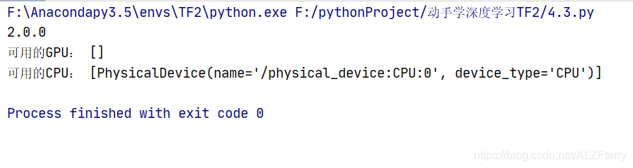
目前我的电脑只装了 CPU
from tensorflow.python.client import device_lib
print(device_lib.list_local_devices())
使用tf.device()来指定特定设备(GPU/CPU)
with tf.device('GPU:0'):
    a = tf.constant([1,2,3],dtype=tf.float32)
    b = tf.random.uniform((3,))
    print(tf.exp(a + b) * 2)
tf.Tensor([12.172885 19.682476 53.18001 ], shape=(3,), dtype=float32)