11_Training Deep Neural Networks_VarianceScaling_leaky relu_PReLU_SELU _Batch Normalization_Reusing
https://blog.csdn.net/Linli522362242/article/details/106935910
11_Training Deep Neural Networks_2_transfer learning_RBMs_Momentum_Nesterov Accelerated Gra_AdaGrad_RMSProp
https://blog.csdn.net/Linli522362242/article/details/106982127
11_Training Deep Neural Networks_3_Adam_Learning Rate Scheduling_Decay_np.argmax(」)_lambda语句_Regular
https://blog.csdn.net/Linli522362242/article/details/107086444
Dropout
Dropout is one of the most popular regularization techniques for deep neural networks. It was proposed in a paper23 by Geoffrey Hinton in 2012 and further detailed in a 2014 paper24 by Nitish Srivastava et al., and it has proven to be highly successful: even the state-of-the-art neural networks get a 1–2% accuracy boost simply by adding dropout. This may not sound like a lot, but when a model already has 95% accuracy, getting a 2% accuracy boost means dropping the error rate by almost 40% (going from 5% error to roughly 3%).
It is a fairly simple algorithm: at every training step, every neuron (including the input neurons, but always excluding the output neurons) has a probability p of being temporarily “dropped out,” meaning it will be entirely ignored during this training step, but it may be active during the next step (see Figure 11-9). The hyperparameter p is called the dropout rate, and it is typically set between 10% and 50%: closer to 20–30% in recurrent递归 neural nets (see Chapter 15), and closer to 40–50% in convolutional neural networks (see Chapter 14). After training, neurons don’t get dropped anymore. And that’s all (except for a technical detail we will discuss momentarily[ˌmoʊmənˈterəli]马上,立刻).
 Figure 11-9. With dropout regularization, at each training iteration a random subset of all neurons in one or more layers—except the output layer—are “dropped out”; these neurons output 0 at this iteration (represented by the dashed arrows)
@tf_export("nn.dropout", v1=[])
def dropout_v2(x, rate, noise_shape=None, seed=None, name=None):
  """Computes dropout: randomly sets elements to zero to prevent overfitting.
  Note: The behavior of dropout has changed between TensorFlow 1.x and 2.x.
  When converting 1.x code, please use named arguments to ensure behavior stays
  consistent.
  See also: `tf.keras.layers.Dropout` for a dropout layer.
  [Dropout](https://arxiv.org/abs/1207.0580) is useful for regularizing DNN
  models. Inputs elements are randomly set to zero (and the other elements are
  rescaled). This encourages each node to be independently useful, as it cannot
  rely on the output of other nodes.
  More precisely: With probability `rate` elements of `x` are set to `0`.
  The remaining elements are scaled up by `1.0 / (1 - rate)`, so that the
  expected value is preserved.

  >>> tf.random.set_seed(0)
  >>> x = tf.ones([3,5])
  >>> tf.nn.dropout(x, rate = 0.5, seed = 1).numpy()# x*1/(1-0.5)
  array([[2., 0., 0., 2., 2.],
       [2., 2., 2., 2., 2.],
       [2., 0., 2., 0., 2.]], dtype=float32)
  >>> tf.random.set_seed(0)
  >>> x = tf.ones([3,5])
  >>> tf.nn.dropout(x, rate = 0.8, seed = 1).numpy()
  array([[0., 0., 0., 5., 5.],
       [0., 5., 0., 5., 0.],
       [5., 0., 5., 0., 5.]], dtype=float32)
  >>> tf.nn.dropout(x, rate = 0.0) == x
  <tf.Tensor: shape=(3, 5), dtype=bool, numpy=
    array([[ True,  True,  True,  True,  True],
           [ True,  True,  True,  True,  True],
           [ True,  True,  True,  True,  True]])>
  By default, each element is kept or dropped independently.  If `noise_shape`
  is specified, it must be
  [broadcastable](http://docs.scipy.org/doc/numpy/user/basics.broadcasting.html)
  to the shape of `x`, and only dimensions with `noise_shape[i] == shape(x)[i]`
  will make independent decisions. This is useful for dropping whole
  channels from an image or sequence. For example:
  >>> tf.random.set_seed(0)
  >>> x = tf.ones([3,10]) #2/3 >0.5
  >>> tf.nn.dropout(x, rate = 2/3, noise_shape=[1,10], seed=1).numpy()
  array([[0., 0., 0., 3., 3., 0., 3., 3., 3., 0.],
       [0., 0., 0., 3., 3., 0., 3., 3., 3., 0.],
       [0., 0., 0., 3., 3., 0., 3., 3., 3., 0.]], dtype=float32)
  Args:
    x: A floating point tensor.
    rate: A scalar `Tensor` with the same type as x. The probability
      that each element is dropped. For example, setting rate=0.1 would drop
      10% of input elements.
    noise_shape: A 1-D `Tensor` of type `int32`, representing the
      shape for randomly generated keep/drop flags.
    seed: A Python integer. Used to create random seeds. See
      `tf.random.set_seed` for behavior.
    name: A name for this operation (optional).
  Returns:
    A Tensor of the same shape of `x`.
  Raises:
    ValueError: If `rate` is not in `[0, 1)` or if `x` is not a floating point
      tensor. `rate=1` is disallowed, because theoutput would be all zeros,
      which is likely not what was intended.
  """
  with ops.name_scope(name, "dropout", [x]) as name:
    is_rate_number = isinstance(rate, numbers.Real)
    if is_rate_number and (rate < 0 or rate >= 1):
      raise ValueError("rate must be a scalar tensor or a float in the "
                       "range [0, 1), got %g" % rate)
    x = ops.convert_to_tensor(x, name="x") #droppout rate
    x_dtype = x.dtype
    if not x_dtype.is_floating:
      raise ValueError("x has to be a floating point tensor since it's going "
                       "to be scaled. Got a %s tensor instead." % x_dtype)
    is_executing_eagerly = context.executing_eagerly()
    if not tensor_util.is_tensor(rate):
      if is_rate_number:
        keep_prob = 1 - rate       #keep probability
        scale = 1 / keep_prob
        scale = ops.convert_to_tensor(scale, dtype=x_dtype)
        ret = gen_math_ops.mul(x, scale) #x/ (1-droppout rate)######################
      else:
        raise ValueError("rate is neither scalar nor scalar tensor %r" % rate)
    else:
      rate.get_shape().assert_has_rank(0)
      rate_dtype = rate.dtype
      if rate_dtype != x_dtype:
        if not rate_dtype.is_compatible_with(x_dtype):
          raise ValueError(
              "Tensor dtype %s is incomptaible with Tensor dtype %s: %r" %
              (x_dtype.name, rate_dtype.name, rate))
        rate = gen_math_ops.cast(rate, x_dtype, name="rate")
      one_tensor = constant_op.constant(1, dtype=x_dtype)
      ret = gen_math_ops.real_div(x, gen_math_ops.sub(one_tensor, rate))

    noise_shape = _get_noise_shape(x, noise_shape)
    # Sample a uniform distribution on [0.0, 1.0) and select values larger
    # than rate.
    #
    # NOTE: Random uniform can only generate 2^23 floats on [1.0, 2.0)
    # and subtract 1.0.
    random_tensor = random_ops.random_uniform(
        noise_shape, seed=seed, dtype=x_dtype)
    # NOTE: if (1.0 + rate) - 1 is equal to rate, then that float is selected,
    # hence a >= comparison is used.
    keep_mask = random_tensor >= rate
    ret = gen_math_ops.mul(ret, gen_math_ops.cast(keep_mask, x_dtype))
    if not is_executing_eagerly:
      ret.set_shape(x.get_shape())
    return ret
It’s surprising at first that this destructive[dɪˈstrʌktɪv]破坏性的 technique works at all. Would a company perform better if its employees were told to toss a coin every morning to decide whether or not to go to work? Well, who knows; perhaps it would! The company would be forced to adapt its organization组织构架; it could not rely on any single person to work the coffee machine or perform any other critical tasks, so this expertise专门知识或技能 would have to be spread across several people. Employees would have to learn to cooperate with many of their coworkers, not just a handful of them. The company would become much more resilient有弹性的. If one person quit, it wouldn’t make much of a difference. It’s unclear whether this idea would actually work for companies, but it certainly does for neural networks. Neurons trained with dropout cannot co-adapt共同适应 with their neighboring neurons; they have to be as useful as possible on their own. They also cannot rely excessively过度地 on just a few input neurons; they must pay attention to each of their input neurons. They end up being less sensitive to slight changes in the inputs. In the end, you get a more robust network that generalizes better.
Another way to understand the power of dropout is to realize that a unique neural network is generated at each training step. Since each neuron can be either present or absent, there are a total of ![]() possible networks (where N is the total number of droppable neurons). This is such a huge number that it is virtually impossible for the same neural network to be sampled twice. Once you have run 10,000 training steps, you have essentially trained 10,000 different neural networks (each with just one training instance). These neural networks are obviously not independent because they share many of their weights, but they are nevertheless all different. The resulting neural network can be seen as an averaging ensemble of all these smaller neural networks.
possible networks (where N is the total number of droppable neurons). This is such a huge number that it is virtually impossible for the same neural network to be sampled twice. Once you have run 10,000 training steps, you have essentially trained 10,000 different neural networks (each with just one training instance). These neural networks are obviously not independent because they share many of their weights, but they are nevertheless all different. The resulting neural network can be seen as an averaging ensemble of all these smaller neural networks.
In practice, you can usually apply dropout only to the neurons in the top one to three layers (excluding the output layer).
There is one small but important technical detail. Suppose p = 50%, in which case during testing a neuron would be connected to twice as many input neurons as it would be (on average) during training. To compensate for this fact, we need to multiply each neuron’s input connection weights by 0.5 after training. If we don’t, each neuron will get a total input signal roughly twice as large as what the network was trained on and will be unlikely to perform well. More generally, we need to multiply each input connection weight by the keep probability (1 – p) after training. Alternatively, we can divide each neuron’s output by the keep probability during training (these alternatives are not perfectly equivalent, but they work equally well).
To implement dropout using Keras, you can use the keras.layers.Dropout layer. During training, it randomly drops some inputs (setting them to 0) and divides the remaining inputs by the keep probability(remaining input/1-rate). After training, it does nothing at all; it just passes the inputs to the next layer.
The following code applies dropout regularization before every Dense layer, using a dropout rate of 0.2:

model = keras.models.Sequential([
    keras.layers.Flatten(input_shape=[28,28]),

    keras.layers.Dropout(rate=0.2),
    keras.layers.Dense(300, activation="elu", kernel_initializer="he_normal"),

    keras.layers.Dropout(rate=0.2),
    keras.layers.Dense(100, activation="elu", kernel_initializer="he_normal"),

    keras.layers.Dropout(rate=0.2),
    keras.layers.Dense(10, activation="softmax")
])

model.compile( loss="sparse_categorical_crossentropy", optimizer="nadam", metrics=["accuracy"])
n_epochs=2
history = model.fit( X_train_scaled, y_train, epochs=n_epochs,
                     validation_data = (X_valid_scaled, y_valid))
Since dropout is only active during training, comparing the training loss and the validation loss can be misleading. In particular, a model may be overfitting the training set and yet have similar training and validation losses. So make sure to evaluate the training loss without dropout (e.g., after training).
If you observe that the model is overfitting, you can increase the dropout rate. Conversely, you should try decreasing the dropout rate if the model underfits the training set. It can also help to increase the dropout rate for large layers, and reduce it for small ones. Moreover, many state-of-the-art architectures only use dropout after the last hidden layer, so you may want to try this if full dropout is too strong.
If you want to regularize a self-normalizing network based on the SELU activation function (as discussed earlier), you should use alpha dropout: this is a variant of dropout that preserves the mean and standard deviation of its inputs (it was introduced in the same paper as SELU, as regular dropout would break self-normalization
https://blog.csdn.net/Linli522362242/article/details/106935910).
Equation 11-5. Nesterov Accelerated Gradient algorithm
Alpha Dropout
Alpha Dropout is a Dropout that keeps mean and variance of inputs to their original values, in order to ensure the self-normalizing property even after this dropout. Alpha Dropout fits well to Scaled Exponential Linear Units by randomly setting activations to the negative saturation value.
rate: float, drop probability (as with Dropout). The multiplicative noise will have standard deviation sqrt(rate / (1 - rate)).
@keras_export('keras.layers.AlphaDropout')
class AlphaDropout(Layer):
  """Applies Alpha Dropout to the input.
  Alpha Dropout is a `Dropout` that keeps mean and variance of inputs
  to their original values, in order to ensure the self-normalizing property
  even after this dropout.
  Alpha Dropout fits well to Scaled Exponential Linear Units
  by randomly setting activations to the negative saturation value.
  Arguments:
    rate: float, drop probability (as with `Dropout`).
      The multiplicative noise will have
      standard deviation `sqrt(rate / (1 - rate))`.
    seed: A Python integer to use as random seed.
  Call arguments:
    inputs: Input tensor (of any rank).
    training: Python boolean indicating whether the layer should behave in
      training mode (adding dropout) or in inference mode (doing nothing).
  Input shape:
    Arbitrary. Use the keyword argument `input_shape`
    (tuple of integers, does not include the samples axis)
    when using this layer as the first layer in a model.
  Output shape:
    Same shape as input.
  """

  def __init__(self, rate, noise_shape=None, seed=None, **kwargs):
    super(AlphaDropout, self).__init__(**kwargs)
    self.rate = rate
    self.noise_shape = noise_shape
    self.seed = seed
    self.supports_masking = True

  def _get_noise_shape(self, inputs):
    return self.noise_shape if self.noise_shape else array_ops.shape(inputs)

  def call(self, inputs, training=None):
    if 0. < self.rate < 1.:
      noise_shape = self._get_noise_shape(inputs)

      def dropped_inputs(inputs=inputs, rate=self.rate, seed=self.seed):  # pylint: disable=missing-docstring
        alpha = 1.6732632423543772848170429916717
        scale = 1.0507009873554804934193349852946
        alpha_p = -alpha * scale

        kept_idx = math_ops.greater_equal(
            K.random_uniform(noise_shape, seed=seed), rate)
        kept_idx = math_ops.cast(kept_idx, inputs.dtype)

        # Get affine transformation params
        a = ((1 - rate) * (1 + rate * alpha_p**2))**-0.5
        b = -a * alpha_p * rate

        # Apply mask
        x = inputs * kept_idx + alpha_p * (1 - kept_idx)

        # Do affine transformation
        return a * x + b

      return K.in_train_phase(dropped_inputs, inputs, training=training)
    return inputs
import tensorflow as tf
import numpy as np

tf.random.set_seed(42)
np.random.seed(42)


model = keras.models.Sequential([
    keras.layers.Flatten( input_shape=[28,28]),

    keras.layers.AlphaDropout( rate=0.2 ),
    keras.layers.Dense(300, activation="selu", kernel_initializer="lecun_normal"),

    keras.layers.AlphaDropout( rate=0.2 ),
    keras.layers.Dense(100, activation="selu", kernel_initializer="lecun_normal"),

    keras.layers.AlphaDropout( rate=0.2 ),
    keras.layers.Dense(10, activation="softmax")
])

optimizer = keras.optimizers.SGD( lr=0.01, momentum=0.9, nesterov=True)
model.compile( loss="sparse_categorical_crossentropy", optimizer=optimizer, metrics=["accuracy"])
n_epochs=20
history = model.fit(X_train_scaled, y_train, epochs=n_epochs,
validation_data=(X_valid_scaled, y_valid)) 
... ...
Since dropout is only active during training, comparing the training loss and the validation loss can be misleading
train loss > val_loss, undefitting, Don't be misslead ![]()
![]() reallly?
reallly?
model.evaluate(X_test_scaled, y_test)
model.evaluate(X_train_scaled, y_train) 
train loss < test loss, overfitting
history = model.fit(X_train_scaled, y_train) ![]()
Monte Carlo (MC) Dropout
In 2016, a paper by Yarin Gal and Zoubin Ghahramani added a few more good reasons to use dropout:
- First, the paper established a profound意义深远的 connection between dropout networks (i.e., neural networks containing a Dropout layer before every weight layer) and approximate Bayesian inference, giving dropout a solid mathematical justification.
- Second, the authors introduced a powerful technique called MC Dropout, which can boost the performance of any trained dropout model without having to retrain it or even modify it at all, provides a much better measure of the model’s uncertainty, and is also amazingly simple to implement.
If this all sounds like a “one weird trick” advertisement, then take a look at the following code. It is the full implementation of MC Dropout, boosting the dropout model we trained earlier without retraining it:
import tensorflow as tf
import numpy as np

tf.random.set_seed(42)
np.random.seed(42)

model = keras.models.Sequential([
    keras.layers.Flatten( input_shape=[28,28]),

    keras.layers.AlphaDropout( rate=0.2 ),
    keras.layers.Dense(300, activation="selu", kernel_initializer="lecun_normal"),

    keras.layers.AlphaDropout( rate=0.2 ),
    keras.layers.Dense(100, activation="selu", kernel_initializer="lecun_normal"),

    keras.layers.AlphaDropout( rate=0.2 ),
    keras.layers.Dense(10, activation="softmax")
])

optimizer = keras.optimizers.SGD( lr=0.01, momentum=0.9, nesterov=True)
model.compile( loss="sparse_categorical_crossentropy", optimizer=optimizer, metrics=["accuracy"])
n_epochs=20
history = model.fit(X_train_scaled, y_train, epochs=n_epochs,
                    validation_data=(X_valid_scaled, y_valid))

#history = model.fit(X_train_scaled, y_train)#without retraining #prediction #??????

y_probas = np.stack([ model(X_test_scaled, training=True) for sample in range(100)])######
We just make 100 predictions over the test set(1000 prediction on each instance), setting training=True to ensure that the Dropout layer is active, and stack the predictions. Since dropout is active, all the predictions will be different. Recall that predict() returns a matrix with one row per instance and one column per class. Because there are 10,000 instances in the test set and 10 classes, this is a matrix of shape [10000, 10]. We stack 100 such matrices, so y_probas is an array of shape [100, 10000, 10].
Once we average over the first dimension (axis=0), we get y_proba, an array of shape [10000, 10], like we would get
with a single prediction. That’s all! Averaging over multiple predictions with dropout on gives us a Monte Carlo estimate that is generally more reliable than the result of a single prediction with dropout off.
y_proba = y_probas.mean(axis=0)
y_std = y_probas.std(axis=0)
For example, let’s look at the model’s prediction for the first instance in the Fashion MNIST test set, with dropout off:
np.round( model.predict(X_test_scaled[:1]),2)![]()
y_test[:1] ![]()
The model seems almost certain that this image belongs to class 9 (ankle boot). Should you trust it? Is there really so little room for doubt? Compare this with the predictions made when dropout is activated:
# y_probas = np.stack([ model(X_test_scaled, training=True) for sample in range(100)])######
np.round(y_probas[:,:1],2)
... ...
This tells a very different story: apparently, when we activate dropout, the model is not sure anymore. It still seems to prefer class 9, but sometimes it hesitates with classes 5 (sandal) and 7 (sneaker), which makes sense given they’re all footwear.
y_probas.shape![]() # number of predictions=100 on the same instance, 10000 instances, 10 class(0~9)
# number of predictions=100 on the same instance, 10000 instances, 10 class(0~9)
y_proba.shape #y_proba = y_probas.mean(axis=0)![]()
y_test.shape![]()
Once we average over the first dimension, we get the following MC Dropout predictions:
np.round( y_proba[:1],2) # #y_proba = y_probas.mean(axis=0)![]()
The model still thinks this image belongs to class 9, but only with a 83% confidence, which seems much more reasonable than 100%###np.round( model.predict(X_test_scaled[:1]),2)###. Plus it’s useful to know exactly which other classes it thinks are likely. And you can also take a look at the standard deviation of the probability estimates:
y_std = y_probas.std(axis=0)
np.round(y_std[:1],2)![]()
Apparently there’s quite a lot of variance in the probability estimates: if you were building a risk-sensitive system (e.g., a medical or financial system), you should probably treat such an uncertain prediction with extreme caution. You definitely would not treat it like a 100% confident prediction. Moreover, the model’s accuracy: 85.8:
y_pred = np.argmax( y_proba, axis=1)
accuracy = np.sum(y_pred == y_test)/len(y_test)
accuracy![]()
The number of Monte Carlo samples you use (100 in this example) is a hyperparameter you can tweak. The higher it is, the more accurate the predictions and their uncertainty estimates will be. However, if you double it, inference time will also be doubled. Moreover, above a certain number of samples, you will notice little improvement. So your job is to find the right trade-off between latency and accuracy, depending on your application.
If your model contains other layers that behave in a special way during training (such as BatchNormalization layers), then you should not force training mode like we just did. Instead, you should replace the Dropout layers with the following MCDropout class:
class MCDropout( keras.layers.Dropout ):
    def call(self, inputs):
        return super().call( inputs, training=True)#######activate dropout
Here, we just subclass the Dropout layer and override the call() method to force its training argument to True (see Chapter 12).
Similarly, you could define an MCAlphaDropout class by subclassing AlphaDropout instead.
If you are creating a model from scratch, it’s just a matter of using MCDropout rather than Dropout. But if you have a
model that was already trained using Dropout, you need to create a new model that’s identical to the existing model except that it replaces the Dropout layers with MCDrop out, then copy the existing model’s weights to your new model.
tf.random.set_seed(42)
np.random.seed(42)

class MCAlphaDropout( keras.layers.AlphaDropout ):
    def call(self, inputs):
        return super().call( inputs, training=True)

# model = keras.models.Sequential([
#     keras.layers.Flatten( input_shape=[28,28]),

#     keras.layers.AlphaDropout( rate=0.2 ),
#     keras.layers.Dense(300, activation="selu", kernel_initializer="lecun_normal"),

#     keras.layers.AlphaDropout( rate=0.2 ),
#     keras.layers.Dense(100, activation="selu", kernel_initializer="lecun_normal"),

#     keras.layers.AlphaDropout( rate=0.2 ),
#     keras.layers.Dense(10, activation="softmax")
# ])

mc_model = keras.models.Sequential([
    MCAlphaDropout( layer.rate ) if isinstance( layer, keras.layers.AlphaDropout ) else layer
    for layer in model.layers
])

mc_model.summary()
optimizer = keras.optimizers.SGD( lr=0.01, momentum=0.9, nesterov=True )
mc_model.compile(loss="sparse_categorical_crossentropy", optimizer=optimizer,
                 metrics=["accuracy"])
mc_model.set_weights(model.get_weights())
# len(model.get_weights()) : 6
len( model.get_weights()[0] ), len( model.get_weights()[1] ), len( model.get_weights()[2] )![]()
len( model.get_weights()[3] ), len( model.get_weights()[4] ), len( model.get_weights()[5] )![]()
Now we can use the model with MC Dropout:
np.round(np.mean([mc_model.predict(X_test_scaled[:1]) for sample in range(100)],
                  axis=0),
2)![]()
In short, MC Dropout is a fantastic technique that boosts dropout models and provides better uncertainty estimates. And of course, since it is just regular dropout during training, it also acts like a regularizer.
Max-Norm Regularization
Another regularization technique that is popular for neural networks is called maxnorm regularization: for each neuron, it constrains the weights w of the incoming connections such that ![]() ≤ r, where r is the max-norm hyperparameter and
≤ r, where r is the max-norm hyperparameter and ![]() is the
is the ![]() norm.
norm.
Max-norm regularization does not add a regularization loss term to the overall loss function. Instead, it is typically implemented by computing ![]() after each training step and rescaling w if needed (w ←
after each training step and rescaling w if needed (w ← ![]() ).
).
Reducing r increases the amount of regularization and helps reduce overfitting. Maxnorm regularization can also help alleviate the unstable gradients problems ###the vanishing/exploding gradients problems during training.
https://blog.csdn.net/Linli522362242/article/details/106935910###(if you are not using Batch Normalization ###This operation simply zero-centers and normalizes each input, then scales and shifts the result using two new parameter vectors per layer: one for scaling, the other for shifting###.
To implement max-norm regularization in Keras, set the kernel_constraint argument of each hidden layer to a max_norm() constraint with the appropriate max value, like this:
layer = keras.layers.Dense( 100, activation="selu", kernel_initializer="lecun_normal",
                            kernel_constraint=keras.constraints.max_norm(1.)
                          )
After each training iteration, the model’s fit() method will call the object returned by max_norm(), passing it the layer’s weights and getting rescaled weights in return, which then replace the layer’s weights. As you’ll see in Chapter 12, you can define your own custom constraint function if necessary and use it as the kernel_constraint. You can also constrain the bias terms by setting the bias_constraint argument.
The max_norm() function has an axis argument that defaults to 0. A Dense layer usually has weights of shape [number of inputs, number of neurons], so using axis=0 means that the max-norm constraint will apply independently to each neuron’s weight vector. If you want to use max-norm with convolutional layers (see Chapter14), make sure to set the max_norm() constraint’s axis argument appropriately (usually axis=[0, 1, 2]).
from functools import partial

MaxNormDense = partial(keras.layers.Dense,
                       activation="selu", kernel_initializer="lecun_normal",
                       kernel_constraint=keras.constraints.max_norm(1.))

model = keras.models.Sequential([
    keras.layers.Flatten(input_shape=[28,28]),
    ##Dense: [number of inputs==784, number of neurons=300]
    MaxNormDense(300),
    MaxNormDense(100),
    keras.layers.Dense(10, activation="softmax")
])
model.compile(loss="sparse_categorical_crossentropy", optimizer="nadam", metrics=["accuracy"])
n_epochs=2
history = model.fit(X_train_scaled, y_train, epochs= n_epochs,
                    validation_data = (X_valid_scaled, y_valid))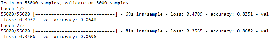
Summary and Practical Guidelines
In this chapter we have covered a wide range of techniques, and you may be wondering which ones you should use. This depends on the task, and there is no clear consensus[kənˈsensəs]舆论; 一致同意 yet, but I have found the configuration in Table 11-3 to work fine in most cases, without requiring much hyperparameter tuning. That said, please do not consider these defaults as hard rules!
Table 11-3. Default DNN configuration
If the network is a simple stack of dense layers, then it can self-normalize, and you should use the configuration in Table 11-4 instead.
Table 11-4. DNN configuration for a self-normalizing net
Don’t forget to normalize the input features! You should also try to reuse parts of a pretrained neural network if you can find one that solves a similar problem, or use unsupervised pretraining if you have a lot of unlabeled data, or use pretraining on an auxiliary task if you have a lot of labeled data for a similar task.
While the previous guidelines should cover most cases, here are some exceptions:
- If you need a sparse model, you can use
 regularization (and optionally zero out the tiny weights after training, https://blog.csdn.net/Linli522362242/article/details/107086444 as discussed in “Lasso Regression” on page 137 in Chapter 4 https://blog.csdn.net/Linli522362242/article/details/104070847 tends to completely eliminate the weights of the least important features最不重要 (i.e., set them to zero) ... since all the weights for the high-degree polynomial features are equal to zero. In other words, Lasso Regression automatically performs feature selection and outputs a sparse model (i.e., with few nonzero feature weights)
- If you need a low-latency model (one that performs lightning-fast predictions), you may need to use fewer layers, fold the Batch Normalization layers into the previous layers, and possibly use a faster activation function such as leaky ReLU or just ReLU. Having a sparse model will also help. Finally, you may want to reduce the float precision from 32 bits to 16 or even 8 bits (see “Deploying a Model to a Mobile or Embedded Device” on page 685). Again, check out TFMOT.
- If you are building a risk-sensitive application, or inference latency is not very important in your application, you can use MC Dropout to boost performance and get more reliable probability estimates, along with uncertainty estimates.
With these guidelines, you are now ready to train very deep nets! I hope you are now convinced that you can go quite a long way using just Keras. There may come a time, however, when you need to have even more control; for example, to write a custom loss function or to tweak the training algorithm. For such cases you will need to use TensorFlow’s lower-level API, as you will see in the next chapter.
Exercises
- Is it OK to initialize all the weights to the same value as long as that value is selected randomly using He initialization?
No, all weights should be sampled independently; they should not all have the same initial value. One important goal of sampling weights randomly is to break symmetry: if all the weights have the same initial value, even if that value is not zero, then symmetry is not broken (i.e., all neurons in a given layer are equivalent), and backpropagation will be unable to break it. Concretely, this means that all the neurons in any given layer will always have the same weights. It’s like having just one neuron per layer, and much slower. It is virtually impossible for such a configuration to converge to a good solution.
- Is it OK to initialize the bias terms to 0?
It is perfectly fine to initialize the bias terms to zero . Some people like to initialize them just like weights, and that’s okay too; it does not make much difference.
- Name three advantages of the SELU activation function over ReLU.
A few advantages of the SELU function over the ReLU function are:
• It can take on negative values, so the average output of the neurons in any given layer is typically closer to zero than when using the ReLU activation function (which never outputs negative values). This helps alleviate the vanishing
gradients problem.
• It always has a nonzero derivative, which avoids the dying units issue that can affect ReLU units.
• When the conditions are right (i.e., if the model is sequential, and the weights are initialized using LeCun initialization, and the inputs are standardized, and there’s no incompatible layer or regularization, such as dropout or ℓ1 regularization), then the SELU activation function ensures the model is selfnormalized, which solves the exploding/vanishing gradients problems.
-
In which cases would you want to use each of the following activation functions: SELU, leaky ReLU (and its variants), ReLU, tanh, logistic, and softmax?
-
The SELU activation function is a good default.
If you need the neural network to be as fast as possible, you can use one of the leaky ReLU variants instead (e.g., a simple leaky ReLU using the default hyperparameter value).
The simplicity of the ReLU activation function makes it many people’s preferred option, despite the fact that it is generally outperformed by SELU and leaky ReLU. However, the ReLU activation function’s ability to output precisely zero can be useful in some cases (e.g., see Chapter 17). Moreover, it can sometimes benefit from optimized implementation as well as from hardware acceleration.
The hyperbolic tangent (tanh) can be useful in the output layer if you need to output a number between –1 and 1, but nowadays it is not used much in hidden layers (except in recurrent nets).
The logistic activation function is also useful in the output layer when you need to estimate a probability (e.g., for binary classification), but is rarely used in hidden layers (there are exceptions—for example, for the coding layer of variational autoencoders; see Chapter 17).
Finally, the softmax activation function is useful in the output layer to output probabilities for mutually exclusive classes, but it is rarely (if ever) used in hidden layers. - What may happen if you set the momentum hyperparameter too close to 1 (e.g., 0.99999) when using an SGD optimizer?
If you set the momentum hyperparameter too close to 1 (e.g., 0.99999) when using an SGD optimizer, then the algorithm will likely pick up a lot of speed, hopefully moving roughly toward the global minimum, but its momentum will carry it right past the minimum. Then it will slow down and come back, accelerate again, overshoot超过 again, and so on. It may oscillate使振荡 this way many times before converging, so overall it will take much longer to converge than with a smaller momentum value.
- Name three ways you can produce a sparse model.
One way to produce a sparse model (i.e., with most weights equal to zero) is to train the model normally, then zero out tiny weights.
For more sparsity, you can apply ℓ1 regularization during training, which pushes the optimizer toward sparsity.
A third option is to use the TensorFlow Model Optimization Toolkit.
- Does dropout slow down training? Does it slow down inference (i.e., making predictions on new instances)? What about MC Dropout?
Yes, dropout does slow down training, in general roughly by a factor of two. However, it has no impact on inference speed since it is only turned on during training.
MC Dropout is exactly like dropout during training, but it is still active during inference, so each inference is slowed down slightly. More importantly, when using MC Dropout you generally want to run inference 10 times or more to get better predictions. This means that making predictions is slowed down by a factor of 10 or more.
- Practice training a deep neural network on the CIFAR10 image dataset:
##############################################
a. Build a DNN with 20 hidden layers of 100 neurons each (that’s too many, but it’s the point of this exercise). Use He initialization and the ELU activation function(SELU > ELU > leaky ReLU (and its variants) > ReLU > tanh > logistic, and question c requires using BN then SELU). ==>HE_normal
https://blog.csdn.net/Linli522362242/article/details/107086444The only difference is that step 1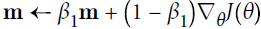 computes an exponentially decaying average rather than an exponentially decaying sum(
 but these are actually equivalent except for a constant factor (the decaying average is just 1 –
  times the decaying sum)., and You can easily verify that if the gradient remains constant, the terminal velocity (i.e., the maximum size of the weight updates, ###Here is m###) is equal to that gradient multiplied by the learning rate η multiplied by 1/(1–β)
https://blog.csdn.net/Linli522362242/article/details/106982127)
##############################################import tensorflow as tf from tensorflow import keras import numpy as np keras.backend.clear_session() tf.random.set_seed(42) np.random.seed(42) model = keras.models.Sequential() model.add( keras.layers.Flatten( input_shape=[32,32,3] ) ) # 32 × 32–pixel color images(255.255.255) for _ in range(20): model.add( keras.layers.Dense(100, activation="elu", kernel_initializer="he_normal") )
b. Using Nadam optimization and early stopping, train the network on the CIFAR10 dataset. You can load it with keras.datasets.cifar10.load_data(). The dataset is composed of 60,000 32 × 32–pixel color images (50,000 for training, 10,000 for testing) with 10 classes, so you’ll need a softmax output layer with 10 neurons. Remember to search for the right learning rate each time you change the model’s architecture or hyperparameters.
https://www.cs.toronto.edu/~kriz/cifar.html
Let's add the output layer to the model: ==> softmax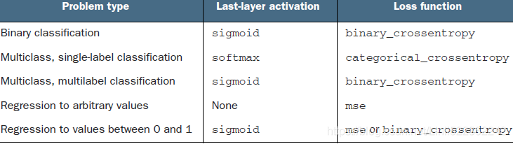
model.add( keras.layers.Dense(10, activation="softmax") )Nadam
- Let's use a Nadam optimizer with a learning rate of 5e-5. I tried learning rates 1e-5, 3e-5, 1e-4, 3e-4, 1e-3, 3e-3 and 1e-2, and I compared their learning curves for 10 epochs each (using the TensorBoard callback, below). The learning rates 3e-5 and 1e-4 were pretty good, so I tried 5e-5, which turned out to be slightly better.
https://blog.csdn.net/Linli522362242/article/details/107086444
Adaptive optimization methods (including RMSProp, Adam, and Nadam optimization) are often great(使用随着loss接近最小值而减小的动态学习率), converging fast to a good solution.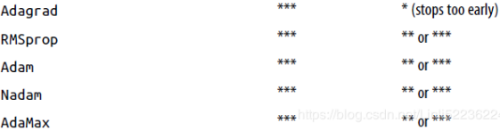
general Adam(结合了Adagrad善于处理稀疏梯度和RMSprop善于处理非平稳目标的优点) performs better than AdaMax(this is just one more optimizer you can try if you experience problems with Adam on some task)
Nadam optimization is Adam optimization plus the Nesterov trick, so it will often converge slightly faster than Adam.
Let's load the CIFAR10 dataset. We also want to use early stopping(since the cost function is convex), so we need a validation set. Let's use the first 5,000 images of the original training set as the validation set(early stopping will interrupt training when it measures no progress on the validation set for a number of epochs (defined by the patience argument ###Number of epochs with no improvement after which training will be stopped.### )optimizer = keras.optimizers.Nadam(lr=5e-5) model.compile( loss="sparse_categorical_crossentropy", optimizer = optimizer, metrics=['accuracy'] )# You can load it with keras.datasets.cifar10.load_data(). The dataset is composed of 60,000 32 × 32–pixel color # images (50,000 for training, 10,000 for testing) with 10 classes, (X_train_full, y_train_full), (X_test, y_test) = keras.datasets.cifar10.load_data() X_train = X_train_full[5000:] y_train = y_train_full[5000:] X_valid = X_train_full[:5000] y_valid = y_train_full[:5000]
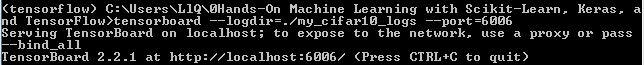
Now we can create the callbacks (in case your computer crashes, the ModelCheckpoint callback回调 saves checkpoints of your model at regular intervals during training, by default at the end of each epoch:) we need and train the model:
# https://www.tensorflow.org/api_docs/python/tf/keras/callbacks/ModelCheckpoint
# mode = "auto"
# 在save_best_only=True时决定性能最佳模型的评判准则,例如,当监测值为val_acc时,模式应为max,
# 当检测值为val_loss时,模式应为min。在auto模式下 mode='auto',评价准则由被监测值的名字自动推断
https://blog.csdn.net/Linli522362242/article/details/106582512early_stopping_cb = keras.callbacks.EarlyStopping(patience=20) # https://www.tensorflow.org/api_docs/python/`tf/keras/callbacks/ModelCheckpoint # mode = "auto" # monitor='val_loss' #default model_checkpoint_cb = keras.callbacks.ModelCheckpoint("my_cifar10_model.h5", save_best_only=True) run_index = 1 # increment every time you train the model import os run_logdir = os.path.join( os.curdir, "my_cifar10_logs", "run_{:03d}".format(run_index) ) tensorboard_cb = keras.callbacks.TensorBoard(run_logdir) callbacks = [early_stopping_cb, model_checkpoint_cb, tensorboard_cb] model.fit( X_train, y_train, epochs=100, validation_data=(X_valid, y_valid), callbacks=callbacks)
... ...
... ...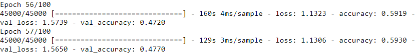
model = keras.models.load_model("my_cifar10_model.h5")
model.evaluate(X_valid, y_valid)
The model with the lowest validation loss gets about 47% accuracy on the validation set. It took 36 epochs to reach the lowest validation loss. Let's see if we can improve performance using Batch Normalization.


The model with the lowest validation loss gets about 47% accuracy on the validation set. It took 36 epochs to reach the lowest validation loss.K = keras.backend class ExponentialLearningRate( keras.callbacks.Callback): def __init__(self, factor): self.factor = factor self.rates = [] self.losses = [] def on_batch_end(self, batch, logs): self.rates.append( K.get_value(self.model.optimizer.lr) ) self.losses.append( logs['loss'] ) K.set_value( self.model.optimizer.lr, self.model.optimizer.lr*self.factor )#update learning rate def find_learing_rate( model, X,y, epochs=1, batch_size=32, min_rate=10**-5, max_rate=10): init_weights = model.get_weights() iterations = len(X) // batch_size * epochs factor = np.exp(np.log(max_rate / min_rate)/iterations) # initilize learning rate factor init_lr = K.get_value(model.optimizer.lr) # get initial learning rate K.set_value( model.optimizer.lr, min_rate ) # replace initial learning rate with min_rate exp_lr = ExponentialLearningRate(factor) # pass learning rate factor to history = model.fit( X, y, epochs=epochs, batch_size=batch_size, callbacks=[exp_lr] ) K.set_value( model.optimizer.lr, init_lr ) # replace current learning rate with initiallearning rate model.set_weights(init_weights) return exp_lr.rates, exp_lr.losses def plot_lr_vs_loss( rates, losses ): plt.plot(rates, losses) plt.gca().set_xscale("log") plt.hlines( min(losses), min(rates),max(rates) ) plt.axis( [min(rates), max(rates), min(losses), (losses[0]+min(losses))/2 ]) plt.xlabel("Learning rate") plt.ylabel("Loss") rates, losses = find_learing_rate( model, X_train, y_train, epochs=1)#default batch_size=32
import matplotlib.pyplot as plt

plot_lr_vs_loss(rates, losses)
(suggestion: do not choose the learning rate when losses arrive the minimum)<--How Do You Find A Good Learning Rate<--https://sgugger.github.io/how-do-you-find-a-good-learning-rate.html 在实践中也可以发现,确定lr更重要的是确定量级,如1e-3和1e-2
###Let's use a Nadam optimizer with a learning rate of 5e-5. I tried learning rates 1e-5, 2e-5, 1e-4, 3e-4, 1e-3, 3e-3 and 1e-2, and I compared their learning curves for 10 epochs each (using the TensorBoard callback, below). The learning rates 2e-5 and 1e-4 were pretty good, so I tried 5e-5, which turned out to be slightly better.###
Let's see if we can improve performance using Batch Normalization.
############################################## -
Batch Normalization
-
c. Now try adding Batch Normalization and compare the learning curves: Is it converging faster than before? Does it produce a better model? How does it affect training speed?
The code below is very similar to the code above, with a few changes:
* I added a BN layer after every Dense layer (before the activation function, SELU > ELU > leaky ReLU (and its variants) > ReLU > tanh > logistic), except for the output layer. I also added a BN layer before the first hidden layer(Machine Learning algorithms don’t perform well when the input numerical attributes have very different scales. the input numerical attributes have very different scales, standardization is much less affected by outliers
https://blog.csdn.net/Linli522362242/article/details/106582512).
* I changed the learning rate to 5e-4. I experimented with 1e-5, 3e-5, 5e-5, 1e-4, 3e-4, 5e-4, 1e-3 and 3e-3, and I chose the one with the best validation performance after 20 epochs.
* I renamed the run directories to run bn* and the model file name to my_cifar10_bn_model.h5keras.backend.clear_session() tf.random.set_seed(42) np.random.seed(42) model = keras.models.Sequential() model.add( keras.layers.Flatten(input_shape=[32, 32, 3]) ) model.add( keras.layers.BatchNormalization() ) for _ in range(20): model.add( keras.layers.Dense(100, kernel_initializer="he_normal") )########## model.add( keras.layers.BatchNormalization() ) ########## model.add( keras.layers.Activation("elu") ) ########## model.add( keras.layers.Dense(10, activation="softmax") ) optimizer = keras.optimizers.Nadam( lr=5e-4 ) ########## model.compile( loss="sparse_categorical_crossentropy", optimizer=optimizer, metrics=['accuracy'] ) early_stopping_cb = keras.callbacks.EarlyStopping(patience=20) model_checkpoint_cb = keras.callbacks.ModelCheckpoint("my_cifar10_bn_model.h5", save_best_only=True) run_index = 1 # increment every time you train the model run_logdir = os.path.join( os.curdir, "my_cifar10_logs", "run_bn_{:03d}".format(run_index) ) tensorboard_cb = keras.callbacks.TensorBoard( run_logdir ) callbacks = [early_stopping_cb, model_checkpoint_cb, tensorboard_cb] model.fit(X_train, y_train, epochs=100, validation_data=(X_valid, y_valid), callbacks=callbacks) model = keras.models.load_model("my_cifar10_bn_model.h5") model.evaluate(X_valid, y_valid)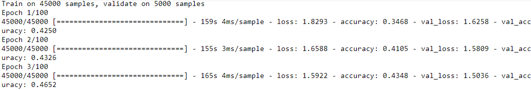
... ...
... ...
Is the model converging faster than before?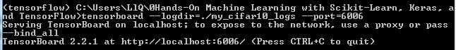

Much faster! The previous model took 36/37 epochs to reach the lowest validation loss, while the new model with BN took 18 epochs. That's more than twice as fast as the previous model. The BN layers stabilized training and allowed us to use a much larger learning rate, so convergence was faster.
Does BN produce a better model?
Yes! The final model is also much better, with 54.2% accuracy instead of 47%. It's still not a very good model, but at least it's much better than before (a Convolutional Neural Network would do much better, but that's a different topic, see chapter 14).
How does BN affect training speed?
Although the model converged twice as fast, each epoch took more time, because of the extra computations required by the BN layers. So overall, although the number of epochs was reduced by 50%, the training time (wall time) was shortened. Which is still pretty significant!
I changed the learning rate to 5e-4. I experimented with 1e-5, 3e-5, 5e-5, 1e-4, 3e-4, 5e-4, 1e-3 and 3e-3, and I chose the one with the best validation performance after 20 epochs.rates, losses = find_learing_rate( model, X_train, y_train, epochs=1) plot_lr_vs_loss(rates, losses)
############################################## -
SELU
-
d. Try replacing Batch Normalization with SELU, and make the necessary adjustements to ensure the network self-normalizes (i.e., standardize the input features, use LeCun normal initialization, make sure the DNN contains only a sequence of dense layers, etc.).
keras.backend.clear_session()
tf.random.set_seed(42)
np.random.seed(42)

model = keras.models.Sequential()
model.add( keras.layers.Flatten(input_shape=[32, 32, 3]) )

for _ in range(20):
    model.add( keras.layers.Dense(100, kernel_initializer="lecun_normal", activation="selu") )#for selu

model.add( keras.layers.Dense(10, activation="softmax") )

optimizer = keras.optimizers.Nadam( lr=5e-4 )                           ##########
model.compile( loss="sparse_categorical_crossentropy",
               optimizer=optimizer,
               metrics=['accuracy']
             )

early_stopping_cb = keras.callbacks.EarlyStopping(patience=20)
model_checkpoint_cb = keras.callbacks.ModelCheckpoint("my_cifar10_selu_model.h5", save_best_only=True)######
run_index = 1 # increment every time you train the model
run_logdir = os.path.join( os.curdir, "my_cifar10_logs", "run_selu_{:03d}".format(run_index) )        ######
tensorboard_cb = keras.callbacks.TensorBoard( run_logdir )
callbacks = [early_stopping_cb, model_checkpoint_cb, tensorboard_cb]

X_means = X_train.mean(axis=0)#for each instances                       #for selu
X_stds = X_train.std(axis=0)
X_train_scaled = (X_train-X_means) /X_stds
X_valid_scaled = (X_valid-X_means) /X_stds
X_test_scaled = (X_test-X_means) /X_stds

model.fit(X_train_scaled, y_train, epochs=100,                         #####
          validation_data=(X_valid_scaled, y_valid),
          callbacks=callbacks)

model = keras.models.load_model("my_cifar10_selu_model.h5")            #####
model.evaluate(X_valid_scaled, y_valid)                                #####
... ...
... ...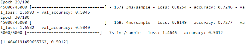
optimizer = keras.optimizers.Nadam( lr=5e-4 ) ##########We get 50.12% accuracy, which is better than the original model, but not quite as good as the model using batch normalization. Moreover, it took 10 epochs to reach the best model, which is much faster than both the original model and the BN model. So it's by far the fastest model to train (both in terms of epochs and wall time).

# optimizer = keras.optimizers.Nadam( lr=7e-4 ) ########### optimizer = keras.optimizers.Nadam( lr=7e-4 ) ########## model = keras.models.load_model("my_cifar10_selu_model.h5") model.evaluate(X_valid_scaled, y_valid)

After compared two loss curves with different learning rate, I believed lr=5e-4 was better than lr=7e-4 since the constraint speed and more lower losses(the difference was not two much# optimizer = keras.optimizers.Nadam( lr=7e-4 ) ########## rates, losses = find_learing_rate( model, X_train_scaled, y_train, epochs=1) plot_lr_vs_loss(rates, losses)

# optimizer = keras.optimizers.Nadam( lr=9e-4 ) ##########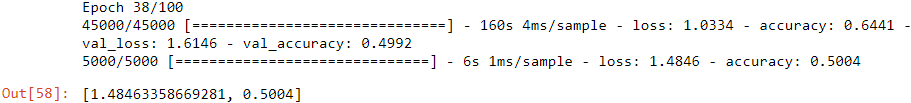
# optimizer = keras.optimizers.Nadam( lr=9e-4 )                           ##########
model = keras.models.load_model("my_cifar10_selu_model.h5")
model.evaluate(X_valid_scaled, y_valid)
rates, losses = find_learing_rate( model, X_train_scaled, y_train, epochs=1)
plot_lr_vs_loss(rates, losses)


Proved: 确定lr更重要的是确定量级,如1e-3和1e-2,因为确定了量级别就一定会constraint, 然后确定lr=5e-4的factor,constraint speed
############################################## -
alpha dropout
-
e. Try regularizing the model with alpha dropout. Then, without retraining your model, see if you can achieve better accuracy using MC Dropout.
keras.backend.clear_session()
tf.random.set_seed(42)
np.random.seed(42)

model = keras.models.Sequential()
model.add(keras.layers.Flatten(input_shape=[32,32,3]))
for _ in range(20):
    model.add(keras.layers.Dense(100,
                                 kernel_initializer="lecun_normal",
                                 activation="selu")
             )
model.add( keras.layers.AlphaDropout(rate=0.1) )#######
model.add( keras.layers.Dense(10, activation="softmax") )

optimizer = keras.optimizers.Nadam(lr=5e-4)
model.compile( loss="sparse_categorical_crossentropy",
               optimizer = optimizer,
               metrics = ["accuracy"]
             )

early_stopping_cb = keras.callbacks.EarlyStopping(patience=20)
model_checkpoint_cb = keras.callbacks.ModelCheckpoint("my_cifar10_alpha_dropout_model.h5",
                                                     save_best_only=True)
run_index = 1 # increment every time you train the model
run_logdir = os.path.join(os.curdir, "my_cifar10_logs",
                          "run_alpha_dropout_{:03d}".format(run_index)
                         )
tensorboard_cb = keras.callbacks.TensorBoard(run_logdir)
callbacks = [early_stopping_cb, model_checkpoint_cb, tensorboard_cb]

X_means = X_train.mean(axis=0)
X_stds = X_train.std(axis=0)
X_train_scaled = (X_train-X_means)/X_stds
X_valid_scaled = (X_valid-X_means)/X_stds
X_test_scaled = ( X_test -X_means)/X_stds

model.fit(X_train_scaled, y_train, epochs=100,
          validation_data= (X_valid_scaled, y_valid),
          callbacks=callbacks)
model = keras.models.load_model("my_cifar10_alpha_dropout_model.h5")
model.evaluate(X_valid_scaled, y_valid)
... ...
... ...
The model reaches 48.66% accuracy on the validation set. That's very slightly worse than without dropout (50.12%). With an extensive hyperparameter search, it might be possible to do better (I tried dropout rates of 5%, 10%, 20% and 40%, and learning rates 1e-4, 3e-4, 5e-4, and 1e-3), but probably not much better in this case.
Let's use MC Dropout now. We will need the MCAlphaDropout class we used earlier, so let's just copy it here for convenience:
class MCAlphaDropout(keras.layers.AlphaDropout):
    def call(self, inputs):
        return super().call(inputs, training=True)#######activate dropout

# Now let's create a new model, identical to the one we just trained (with the same weights),
# but with MCAlphaDropout dropout layers instead of AlphaDropout layers:
mc_model = keras.models.Sequential([
    ##############
    MCAlphaDropout(layer.rate) if isinstance(layer, keras.layers.AlphaDropout) else layer
    for layer in model.layers
])

# we don't need the following codes since we using AlphaDropout############
# optimizer = keras.optimizers.Nadam(lr=5e-4)
# mc_model.compile( loss="sparse_categorical_crossentropy",
#                optimizer = optimizer,
#                metrics = ["accuracy"]
#              )

# Then let's add a couple utility functions. The first will run the model many times
# (10 by default) and it will return the mean predicted class probabilities.
def mc_dropout_predict_probas( mc_model, X, n_samples=10):
    #each elem is predictions to X, n_samples predictions(prediction list)
    Y_probas = [mc_model.predict(X) for sample in range(n_samples) ]
    # Y_probas
    # here 0,1,...,9 represent their probabilities
    # [ [ [0,1,...,9], [0,1,...,9], ...len(X)..., [0,1,...,9] ],
    #   [ [0,1,...,9], [0,1,...,9], ...len(X)..., [0,1,...,9] ],
    #     ... ...n_samples
    #   [ [0,1,...,9], [0,1,...,9], ...len(X)..., [0,1,...,9] ],
    # ]
    return np.mean(Y_probas, axis=0)#return[ [0,1,...,9], [0,1,...,9], ...len(X)..., [0,1,...,9] ]

# The second will use these mean probabilities to predict the most likely class for
# each instance:
def mc_dropout_predict_classes( mc_model, X, n_samples=10):
    Y_probas = mc_dropout_predict_probas(mc_model, X, n_samples)
    return np.argmax(Y_probas, axis=1) #return[ 0, 9, ...len(X)..., 8 ]

# Now let's make predictions for all the instances in the validation set,
# and compute the accuracy:
keras.backend.clear_session()
tf.random.set_seed(42)
np.random.seed(42)

# we don't fit function here, since we using Alphal dropout model which has been fit
# model.fit(X_train_scaled, y_train, epochs=100,
#           validation_data= (X_valid_scaled, y_valid),
#           callbacks=callbacks)

y_pred = mc_dropout_predict_classes(mc_model, X_valid_scaled) #without retraining #prediction
accuracy = np.mean(y_pred==y_valid[:,0])# y_valid[:,0]: y_valid.shape==(5000,1)
accuracy ![]()
We only get virtually no accuracy improvement in this case (from 48.66% to 48.62% ![]()
![]()
![]() ).
).
So the best model we got in this exercise is the Batch Normalization model(54.12%).
##############################################
1cycle scheduling
f. Retrain your model using 1cycle scheduling and see if it improves training speed and model accuracy.
keras.backend.clear_session()
tf.random.set_seed(42)
np.random.seed(42)

model = keras.models.Sequential()
model.add( keras.layers.Flatten( input_shape=[32,32,3]) )
for _ in range(20):
    model.add( keras.layers.Dense(100, kernel_initializer="lecun_normal", activation="selu") )

model.add(keras.layers.AlphaDropout(rate=0.1))
model.add(keras.layers.Dense(10, activation="softmax"))

optimizer = keras.optimizers.SGD(lr=1e-3)
model.compile( loss="sparse_categorical_crossentropy",
               optimizer=optimizer,
               metrics=['accuracy'])
K = keras.backend

class ExponentialLearningRate( keras.callbacks.Callback):
    def __init__(self, factor):
        self.factor = factor
        self.rates = []
        self.losses = []

    def on_batch_end(self, batch, logs):
        self.rates.append( K.get_value(self.model.optimizer.lr) )
        self.losses.append( logs['loss'] )
        K.set_value( self.model.optimizer.lr, self.model.optimizer.lr*self.factor )#update learning rate#callbacks

def find_learning_rate( model, X,y, epochs=1, batch_size=32, min_rate=10**-5, max_rate=10):
    init_weights = model.get_weights()

    iterations = len(X) // batch_size * epochs
    factor = np.exp(np.log(max_rate / min_rate)/iterations)
    init_lr = K.get_value(model.optimizer.lr)   # get initial learning rate
    K.set_value( model.optimizer.lr, min_rate ) # replace initial learning rate with min_rate
    exp_lr = ExponentialLearningRate(factor)    # pass learning rate factor to
    history = model.fit( X, y, epochs=epochs, batch_size=batch_size, callbacks=[exp_lr] )
    K.set_value( model.optimizer.lr, init_lr )  # replace current learning rate with initiallearning rate

    model.set_weights(init_weights)
    return exp_lr.rates, exp_lr.losses

def plot_lr_vs_loss( rates, losses ):
    plt.plot(rates, losses)
    plt.gca().set_xscale("log")
    plt.hlines( min(losses), min(rates),max(rates) )
    plt.axis( [min(rates), max(rates),  min(losses), (losses[0]+min(losses))/2 ])
    plt.xlabel("Learning rate")
    plt.ylabel("Loss")
batch_size = 128
#sorry for spelling error, you can correct it, find_learning_rate
rates, losses =find_learning_rate(model, X_train_scaled, y_train, epochs=1, batch_size=batch_size)
plot_lr_vs_loss(rates, losses)
plt.axis([ min(rates), max(rates),
min(losses), (losses[0]+min(losses))/1.4 ])
From learning rate VS Loss curve, the best learing rate is factor*e^-4 ~e^-3
keras.backend.clear_session()
tf.random.set_seed(42)
np.random.seed(42)

model = keras.models.Sequential()
model.add( keras.layers.Flatten( input_shape=[32,32,3] ) )
for _ in range(20):
    model.add(keras.layers.Dense(100,
                                 kernel_initializer="lecun_normal",
                                 activation="selu"))

model.add( keras.layers.AlphaDropout(rate=0.1))
model.add( keras.layers.Dense(10, activation="softmax") )

optimizer = keras.optimizers.SGD( lr=1e-3 ) #from learing rate VS loss curves
model.compile( loss="sparse_categorical_crossentropy",
              optimizer=optimizer,
              metrics=["accuracy"] )
class OneCycleScheduler( keras.callbacks.Callback ):
def __init__(self, iterations, max_rate, start_rate=None,
last_iterations=None, last_rate=None):
self.iterations = iterations #total iterations
self.max_rate = max_rate
self.start_rate = start_rate or max_rate/10
self.last_iterations = last_iterations or iterations//10+1
self.half_iteration_pos = (iterations - self.last_iterations)//2
# finishing the last few epochs by dropping the rate down by several orders of magnitude
self.last_rate = last_rate or self.start_rate/1000
self.iteration_pos = 0
def _iterpolate( self, iter1, iter2,
rate1, rate2):
# a_slope: (rate2-rate1)/(iter2-iter1)
# x: (self.iteration-iter1)
# b: rate1
# y= a_slope * x + b
return ( (rate2-rate1)*(self.iteration_pos-iter1) / (iter2-iter1) + rate1 )
def on_batch_begin(self, batch, logs):
if self.iteration_pos < self.half_iteration_pos:
rate = self._iterpolate(0, self.half_iteration_pos,
self.start_rate, self.max_rate)
elif self.iteration_pos < 2*self.half_iteration_pos:
rate = self._iterpolate(self.half_iteration_pos, 2*self.half_iteration_pos,
self.max_rate, self.start_rate)
else:#last few epochs
rate = self._iterpolate(2*self.half_iteration_pos, self.iterations,
self.start_rate, self.last_rate)
self.iteration_pos +=1
K.set_value(self.model.optimizer.lr, rate)#updaten_epochs = 15
onecycle = OneCycleScheduler( len(X_train_scaled)//batch_size*n_epochs, max_rate=0.02)#max_rate=0.02 from learning rate VS loss curve
history = model.fit(X_train_scaled, y_train, epochs = n_epochs, batch_size=batch_size,
validation_data=(X_valid_scaled, y_valid),
callbacks=[onecycle])
model.evaluate(X_valid_scaled, y_valid)
... ...
One cycle allowed us to train the model in just 15 epochs, each taking only 75 seconds (thanks to the larger batch size). This is over 3 times faster than the fastest model we trained so far. Moreover, we improved the model's performance (from 48.66% to 51%). The batch normalized model reaches a slightly better performance, but it's much slower to train.