11_Training Deep Neural Networks_VarianceScaling_leaky relu_PReLU_SELU _Batch Normalization_Reusing
https://blog.csdn.net/Linli522362242/article/details/106935910
11_Training Deep Neural Networks_2_transfer learning_RBMs_Momentum_Nesterov Accelerated Gra_AdaGrad_RMSProp
https://blog.csdn.net/Linli522362242/article/details/106982127
Adam and Nadam Optimization
Adam, which stands for adaptive moment estimation自适应矩估计, combines the ideas of momentum optimization and RMSProp: just like momentum optimization, it keeps track of an exponentially decaying average of past gradients; and just like RMSProp, it keeps track of an exponentially decaying average of past squared gradients (see Equation 11-8).
Equation 11-8. Adam algorithm
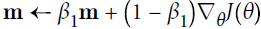 # Momentum algorithm #1
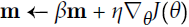
OR # Momentum algorithm 2#1
  note β is negative
 # RMSProp algorithm #1

 # RMSProp algorithm 2#2
OR # RMSProp algorithm 2 #2
- In this equation, t represents the iteration number (starting at 1).
可以看出,直接对梯度的矩估计对内存没有额外的要求,而且可以根据梯度进行动态调整,而![]() 对学习率形成一个动态约束,而且有明确的范围。
对学习率形成一个动态约束,而且有明确的范围。
特点:
- 结合了Adagrad善于处理稀疏梯度和RMSprop善于处理非平稳目标的优点
- 对内存需求较小
- 为不同的参数计算不同的自适应学习率
- 也适用于大多非凸优化- 适用于大数据集和高维空间
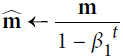
If you just look at steps 1, 2, and 5, you will notice Adam’s close similarity to both momentum optimization and RMSProp. The only difference is that step 1 computes an exponentially decaying average rather than an exponentially decaying sum, but these are actually equivalent except for a constant factor (the decaying average is just ![]() times the decaying sum). Steps 3 and 4 are somewhat of a technical detail: since m and s are initialized at 0, they will be biased toward 0 at the beginning of training, so these two steps will help boost m and s at the beginning of training.
times the decaying sum). Steps 3 and 4 are somewhat of a technical detail: since m and s are initialized at 0, they will be biased toward 0 at the beginning of training, so these two steps will help boost m and s at the beginning of training.
The momentum decay hyperparameter ![]() is typically initialized to 0.9, while the scaling decay hyperparameter
is typically initialized to 0.9, while the scaling decay hyperparameter ![]() is often initialized to 0.999. As earlier, the smoothing term ε is usually initialized to a tiny number such as
is often initialized to 0.999. As earlier, the smoothing term ε is usually initialized to a tiny number such as ![]() . These are the default values for the Adam class (to be precise, epsilon defaults to None, which tells Keras to use keras.backend.epsilon(), which defaults to
. These are the default values for the Adam class (to be precise, epsilon defaults to None, which tells Keras to use keras.backend.epsilon(), which defaults to ![]() ; you can change it using keras.backend.set_epsilon()). Here is how to create an Adam optimizer using Keras:
; you can change it using keras.backend.set_epsilon()). Here is how to create an Adam optimizer using Keras:
optimizer = keras.optimizers.Adam(lr=0.001, beta_1=0.9, beta_2=0.999)Since Adam is an adaptive learning rate algorithm (like AdaGrad and RMSProp), it requires less tuning of the learning rate hyperparameter η. You can often use the default value η = 0.001, making Adam even easier to use than Gradient Descent.
If you are starting to feel overwhelmed[,ovə'welmd]不知所措 by all these different techniques and are wondering how to choose the right ones for your task, don’t worry: some practical guidelines are provided at the end of this chapter.
Finally, two variants of Adam are worth mentioning:
AdaMax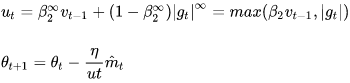
- # Momentum algorithm #1
m_hat = m / (1-beta_1 ** epoch_index) - max (
 ) #OR (
 , abs(
 )
) 
 #here m is m_hat
- Notice that in step 2 of Equation 11-8, Adam accumulates the squares of the gradients
 in s (with a greater weight for more recent gradients). In step 5, if we ignore ε and steps 3 and 4 (which are technical details anyway), Adam scales down the parameter updates by the square root of s. In short, Adam scales down the parameter updates by the ℓ2 norm of the time-decayed gradients (recall that the ℓ2 norm is the square root of the sum of squares). AdaMax, introduced in the same paper as Adam, replaces the ℓ2 norm with the
  norm (a fancy way of saying the max, https://blog.csdn.net/Linli522362242/article/details/103387527, gives the maximum absolute value in the vector). Specifically, it replaces step 2 in Equation 11-8 with s ← max (), it drops step 4, and in step 5 it scales down the gradient updates by a factor of s, which is just the max of the time-decayed gradients. In practice, this can make AdaMax more stable than Adam, but it really depends on the dataset, and in general Adam performs better. So, this is just one more optimizer you can try if you experience problems with Adam on some task.
 class AdaMax(AdaptiveMomentEstimation): def __init__(self, **kwargs): super(AdaMax, self).__init__(**kwargs) def fit(self, X, y): X = np.c_[np.ones(len(X)), X] n_samples, n_features = X.shape self.theta = np.ones(n_features) self.loss_ = [0] m_t = np.zeros(n_features) u_t = np.zeros(n_features) beta_1=0.9, beta_2=0.999 #typically initialized self.i = 0 while self.i < self.n_iter: self.i += 1 if self.shuffle: X, y = self._shuffle(X, y) errors = [] for j in range(0, n_samples, self.batch_size): mini_X, mini_y = X[j: j + self.batch_size], y[j: j + self.batch_size] error = mini_X.dot(self.theta) - mini_y errors.append(error.dot(error)) mini_gradient = 1 / self.batch_size * mini_X.T.dot(error) m_t = self.beta_1 * m_t + (1 - self.beta_1) * mini_gradient m_t_hat = m_t / (1 - self.beta_1 ** self.i)################ u_t = np.max(np.c_[self.beta_2 * u_t, np.abs(mini_gradient)], axis=1) self.theta -= self.eta / u_t * m_t_hat loss = 1 / (2 * self.batch_size) * np.mean(errors) delta_loss = loss - self.loss_[-1] self.loss_.append(loss) if np.abs(delta_loss) < self.tolerance: break return selfNadam
 # the updated theta fomula should be corrected
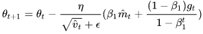
可以看出,Nadam对学习率有了更强的约束,同时对梯度的更新也有更直接的影响。一般而言,在想使用带动量的RMSprop,或者Adam的地方,大多可以使用Nadam取得更好的效果。
- Nadam optimization is Adam optimization plus the Nesterov trick, so it will often converge slightly faster than Adam. In his report introducing this technique, the researcher Timothy Dozat compares many different optimizers on various tasks and finds that Nadam generally outperforms Adam but is sometimes outperformed by RMSProp.
https://zhuanlan.zhihu.com/p/77380412class Nadam(AdaptiveMomentEstimation): def __init__(self, **kwargs): super(Nadam, self).__init__(**kwargs) def fit(self, X, y): X = np.c_[np.ones(len(X)), X] n_samples, n_features = X.shape self.theta = np.ones(n_features) self.loss_ = [0] m_t = np.zeros(n_features) v_t = np.zeros(n_features) beta_1=0.9, beta_2=0.999 #typically initialized #beta_1 should be a list self.i = 0 while self.i < self.n_iter: self.i += 1 if self.shuffle: X, y = self._shuffle(X, y) errors = [] for j in range(0, n_samples, self.batch_size): mini_X, mini_y = X[j: j + self.batch_size], y[j: j + self.batch_size] error = mini_X.dot(self.theta) - mini_y errors.append(error.dot(error)) mini_gradient = 1 / self.batch_size * mini_X.T.dot(error) m_t = self.beta_1 * m_t + (1 - self.beta_1) * mini_gradient m_t_hat = m_t / (1 - self.beta_1 ** self.i) # correction # since self.beta_1**self.i should be the multiplication of current beta_1 list v_t = self.beta_2 * v_t + (1 - self.beta_2) * mini_gradient ** 2 v_t_hat = v_t / (1 - self.beta_2 ** self.i) self.theta -= self.eta / (np.sqrt(v_t_hat) + self.epsilon) * ( self.beta_1 * m_t_hat + (1 - self.beta_1) * mini_gradient / (1 - self.beta_1 ** self.i)) loss = 1 / (2 * self.batch_size) * np.mean(errors) delta_loss = loss - self.loss_[-1] self.loss_.append(loss) if np.abs(delta_loss) < self.tolerance: break return selfAdaptive optimization methods (including RMSProp, Adam, and Nadam optimization) are often great, converging fast to a good solution. However, a 2017 paper###Ashia C. Wilson et al., “The Marginal Value of Adaptive Gradient Methods in Machine Learning,” Advances in Neural Information Processing Systems 30 (2017): 4148–4158.### by Ashia C. Wilson et al. showed that they can lead to solutions that generalize poorly on some datasets. So when you are disappointed by your model’s performance, try using plain Nesterov Accelerated Gradient instead: your dataset may just be allergic to adaptive gradients. Also check out the latest research, because it’s moving fast.
All the optimization techniques discussed so far only rely on the first-order partial derivatives (Jacobians). The optimization literature also contains amazing algorithms based on the second-order partial derivatives (the Hessians, which are the partial
derivatives of the Jacobians). Unfortunately, these algorithms are very hard to apply to deep neural networks because there are ![]() Hessians per output (where n is the number of parameters), as opposed to just n Jacobians per output. Since DNNs typically have tens of thousands of parameters, the second-order optimization algorithms often don’t even fit in memory, and even when they do, computing the Hessians is just too slow.
Hessians per output (where n is the number of parameters), as opposed to just n Jacobians per output. Since DNNs typically have tens of thousands of parameters, the second-order optimization algorithms often don’t even fit in memory, and even when they do, computing the Hessians is just too slow.
经验之谈
- 对于稀疏数据,尽量使用学习率可自适应的优化方法,不用手动调节,而且最好采用默认值
- SGD通常训练时间更长,但是在好的初始化和学习率调度方案的情况下,结果更可靠
- 如果在意更快的收敛,并且需要训练较深较复杂的网络时,推荐使用学习率自适应adaptive learning rate的优化方法。
- Adadelta,RMSprop,Adam是比较相近的算法,在相似的情况下表现差不多。
- 在想使用带动量的RMSprop,或者Adam的地方,大多可以使用Nadam取得更好的效果
#######################################
Training Sparse Models
All the optimization algorithms just presented produce dense密集 models, meaning that most parameters will be nonzero. If you need a blazingly fast model at runtime, or if you need it to take up less memory, you may prefer to end up with a sparse model instead.
One easy way to achieve this is to train the model as usual, then get rid of the tiny weights (set them to zero). Note that this will typically not lead to a very sparse model, and it may degrade the model’s performance.
A better option is to apply strong ℓ1 regularization during training (we will see how later in this chapter), as it pushes the optimizer to zero out as many weights as it can (as discussed in “Lasso Regression” on page 137 in Chapter 4
https://blog.csdn.net/Linli522362242/article/details/104070847 tends to completely eliminate the weights of the least important features最不重要 (i.e., set them to zero) ... since all the weights for the high-degree polynomial features are equal to zero. In other words, Lasso Regression automatically performs feature selection and outputs a sparse model (i.e., with few nonzero feature weights).
If these techniques remain insufficient, check out the TensorFlow Model Optimization Toolkit (TF-MOT), which provides a pruning API capable of iteratively removing connections during training based on their magnitude.
#######################################
Table 11-2 compares all the optimizers we’ve discussed so far (* is bad, ** is average, and *** is good).
Table 11-2. Optimizer comparison
Learning Rate Scheduling
Finding a good learning rate is very important. If you set it much too high, training may diverge (as we discussed in “Gradient Descent” on page 118). If you set it too low, training will eventually converge to the optimum, but it will take a very long time. If you set it slightly too high, it will make progress very quickly at first, but it will end up dancing around the optimum, never really settling down. If you have a limited computing budget, you may have to interrupt training before it has converged properly, yielding a suboptimal solution (see Figure 11-8).
Figure 11-8. Learning curves for various learning rates η
As we discussed in Chapter 10https://blog.csdn.net/Linli522362242/article/details/106849041 One way to find a good learning rate is to train the model for a few hundred iterations, starting with a very low learning rate (e.g.,  ) and gradually increasing it up to a very large value (e.g., 10). This is done by multiplying the learning rate by a constant factor at each iteration (e.g., by
 ![]() =0.03261938194,
=0.03261938194, ![]() ~10 ==>
~10 ==>![]() ) to go from to 10 in 500 iterations). the optimal learning rate will be a bit lower than the point at which the loss starts to climb (typically about 10 times lower than the turning point), you can find a good learning rate by training the model for a few hundred iterations, exponentially increasing the learning rate from a very small value to a very large value, and then looking at the learning curve and picking a learning rate slightly lower than the one at which the learning curve starts shooting back up. You can then reinitialize your model and train it with that learning rate.
) to go from to 10 in 500 iterations). the optimal learning rate will be a bit lower than the point at which the loss starts to climb (typically about 10 times lower than the turning point), you can find a good learning rate by training the model for a few hundred iterations, exponentially increasing the learning rate from a very small value to a very large value, and then looking at the learning curve and picking a learning rate slightly lower than the one at which the learning curve starts shooting back up. You can then reinitialize your model and train it with that learning rate.
But you can do better than a constant learning rate: if you start with a large learning rate and then reduce it once training stops making fast progress, you can reach a good solution faster than with the optimal constant learning rate. There are many different strategies to reduce the learning rate during training. It can also be beneficial to start with a low learning rate, increase it, then drop it again. These strategies are called learning schedules (we briefly introduced this concept in Chapter 4). These are
the most commonly used learning schedules: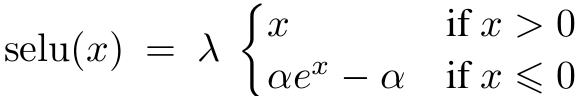
where alpha![]() and
and scale![]() are pre-defined constants (
are pre-defined constants (alpha = 1.67326324 and scale = 1.05070098).
from scipy.special import erfc

# alpha and scale to self normalize with mean 0 and standard deviation 1
# (see equation 14 in the paper https://arxiv.org/pdf/1706.02515.pdf):
alpha_0_1 = -np.sqrt(2/np.pi) / ( erfc(1/np.sqrt(2)) * np.exp(1/2)-1 ) # alpha_0_1 ≈ 1.6732632423543778
scale_0_1 = ( 1- erfc( 1/np.sqrt(2) )*np.sqrt(np.e) ) * np.sqrt( 2*np.pi )*\
            ( 2* erfc( np.sqrt(2) )*np.e**2 + np.pi*erfc(1/np.sqrt(2))**2*np.e \
             -2*(2+np.pi)*erfc( 1/np.sqrt(2) )*np.sqrt(np.e) + np.pi + 2\
            )**(-1/2)  # scale_0_1 ≈ 1.0507009873554805


def selu( z, scale=scale_0_1, alpha=alpha_0_1 ):
    return scale * elu(z,alpha)
https://blog.csdn.net/Linli522362242/article/details/106935910
https://towardsdatascience.com/selu-make-fnns-great-again-snn-8d61526802a9
https://www.tensorflow.org/api_docs/python/tf/keras/activations/selu?hl=ru&authuser=19
- Every hidden layer’s weights must be initialized with LeCun normal initialization. In Keras, this means setting kernel_initializer="lecun_normal".
- The paper only guarantees self-normalization if all layers are dense, but some researchers have noted that the SELU activation function can improve performance in convolutional neural nets as well (see Chapter 14).
from tensorflow import keras

(X_train_full, y_train_full), (X_test, y_test) = keras.datasets.fashion_mnist.load_data()

# scale the pixel intensities down to the 0–1 range by dividing them by 255.0
#(this also converts them to floats)
X_train_full = X_train_full/255.0
X_test = X_test/255.0
X_valid, X_train = X_train_full[:5000], X_train_full[5000:]
y_valid, y_train = y_train_full[:5000], y_train_full[5000:]

# for using Scaled ELU (SELU) activation function
# The input features must be standardized (mean 0 and standard deviation 1).
pixel_means = X_train.mean(axis=0, keepdims=True) # axis=0 for all instances # pixel_means.shape : (1, 28, 28)
pixel_stds = X_train.std(axis=0, keepdims=True) # pixel_stds.shape : (1, 28, 28)
X_train_scaled = (X_train-pixel_means)/pixel_stds
X_valid_scaled = (X_valid-pixel_means)/pixel_stds
X_test_scaled = (X_test - pixel_means)/pixel_stds
Power scheduling幂调度
- Set the learning rate to a function of the iteration number t (#I believe t is steps in keras#): η(t) =
 . The initial learning rate
  , the power c (typically set to 1), and the steps s (#I believe s is decay_steps in keras#) are hyperparameters. The learning rate drops at each step. After t=1 steps and s=1, it is down to / 2. After t=2 steps and s=1, it is down to / 3, then it goes down to / 4, then /5, and so on. As you can see, this schedule first drops quickly, then more and more slowly. Of course, power scheduling requires tuning and s (and possibly c).
 -
momentumbetween 0 (high friction) and 1 (no friction)
The update rule for θ with gradient g when
momentumis 0.0:
The update rule when
momentumis larger than 0.0(β>0): is negative since
  ,有方向gradent是向下(negative),但是在计算机计算过程为了好处理使用了正值
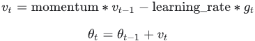
if
Go tonesterovis False, gradient is evaluated at. if nesterovis True, gradient is evaluated at , and the variables always store θ+mv instead of theta
https://www.tensorflow.org/api_docs/python/tf/keras/optimizers/schedules/LearningRateSchedule?hl=ru&authuser=19
Thenget_config ==> View source
https://github.com/tensorflow/tensorflow/blob/v2.2.0/tensorflow/python/keras/optimizer_v2/learning_rate_schedule.py#L46-L48
Go to class InverseTimeDecay
decayed_learning_rate : initial_learning_rate / (1 + decay_rate * steps / decay_steps)@keras_export("keras.optimizers.schedules.InverseTimeDecay") class InverseTimeDecay(LearningRateSchedule): """A LearningRateSchedule that uses an inverse time decay schedule.""" def __init__( self, initial_learning_rate, decay_steps, #default =1 decay_rate, staircase=False, name=None): """Applies inverse time decay to the initial learning rate. ```python def decayed_learning_rate(step): return initial_learning_rate / (1 + decay_rate * steps / decay_steps) ``` or, if `staircase` is `True`, as: ```python def decayed_learning_rate(step): return initial_learning_rate / (1 + decay_rate * floor(steps / decay_steps)) ``` Args: initial_learning_rate: A scalar `float32` or `float64` `Tensor` or a Python number. The initial learning rate. decay_steps: How often to apply decay. decay_rate: A Python number. The decay rate. staircase: Whether to apply decay in a discrete staircase, as opposed to continuous, fashion. name: String. Optional name of the operation. Defaults to 'InverseTimeDecay'. """ super(InverseTimeDecay, self).__init__() self.initial_learning_rate = initial_learning_rate self.decay_steps = decay_steps self.decay_rate = decay_rate self.staircase = staircase self.name = name def __call__(self, step): with ops.name_scope_v2(self.name or "InverseTimeDecay") as name: initial_learning_rate = ops.convert_to_tensor_v2( self.initial_learning_rate, name="initial_learning_rate") dtype = initial_learning_rate.dtype decay_steps = math_ops.cast(self.decay_steps, dtype) decay_rate = math_ops.cast(self.decay_rate, dtype) #initial_learning_rate / (1 + decay_rate * step / decay_step)################### global_step_recomp = math_ops.cast(step, dtype) p = global_step_recomp / decay_steps # steps / decay_steps if self.staircase: p = math_ops.floor(p) const = math_ops.cast(constant_op.constant(1), dtype) # 1 denom = math_ops.add(const, math_ops.multiply(decay_rate, p)) # (1 + decay_rate * step / decay_steps) return math_ops.divide(initial_learning_rate, denom, name=name)# initial_learning_rate / denom
lr = lr0 / ( 1 + steps / s )**c            and  Keras uses c=1, s = decay_steps/decay , decay_steps=1
lr =           lr0         / ( 1 + steps / (decay_steps/decay) ) ^1
lr =           lr0         / ( 1 + steps / (     1     /decay) )
lr =           lr0         / ( 1 + decay      * steps/ 1 )
lr = initial_learning_rate / ( 1 + decay_rate * steps / 1 )
lr = initial_learning_rate / ( 1 + decay_rate * steps / 1 )
lr = initial_learning_rate / ( 1 + decay_rate * steps / 1 )
Implementing power scheduling in Keras is the easiest option: just set the decay hyperparameter when creating an optimizer:
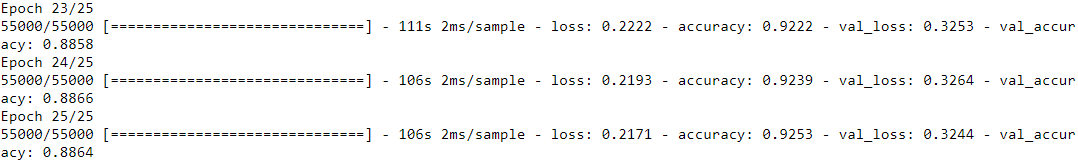
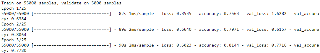
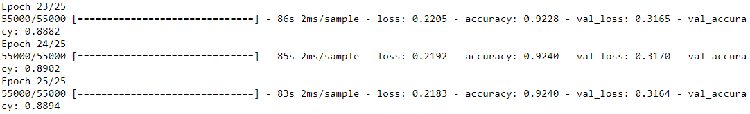
The decay is the inverse of s (the number of steps it takes to divide the learning rate by one more unit), and Keras assumes that c is equal to 1.#class SGD(tensorflow.python.keras.optimizer_v2.optimizer_v2.OptimizerV2) # | SGD(learning_rate=0.01, momentum=0.0, nesterov=False, name='SGD', **kwargs) optimizer = keras.optimizers.SGD( lr=0.01, decay=1e-4) import tensorflow as tf import numpy as np tf.random.set_seed(42) np.random.seed(42) model = keras.models.Sequential([ keras.layers.Flatten(input_shape=[28,28]), # 1D arrray: 28*28 keras.layers.Dense( 300, activation="selu", kernel_initializer="lecun_normal" ),#Scaled ELU keras.layers.Dense( 100, activation="selu", kernel_initializer="lecun_normal" ), keras.layers.Dense( 10, activation="softmax") ]) model.compile(loss="sparse_categorical_crossentropy", optimizer=optimizer, metrics=["accuracy"]) n_epochs=25 history = model.fit( X_train_scaled, y_train, epochs=n_epochs, validation_data=(X_valid_scaled, y_valid) )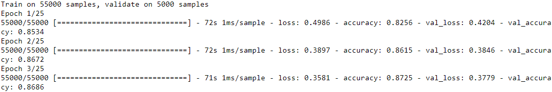
... ...
import matplotlib.pyplot as plt

learning_rate = 0.01
decay = 1e-4
batch_size=32
n_steps_per_epoch = len(X_train) //batch_size
epochs = np.arange(n_epochs)
lrs = learning_rate / (1 + decay* epochs*n_steps_per_epoch )

plt.plot( epochs, lrs, "o-")
plt.axis([0, n_epochs-1, 0, 0.01])
plt.xlabel("Epoch")
plt.ylabel("Learning Rate")
plt.title("Power Scheduling", fontsize=14)
plt.grid(True)
plt.show()
# class SGD(tensorflow.python.keras.optimizer_v2.optimizer_v2.OptimizerV2)
# |  SGD(learning_rate=0.01, momentum=0.0, nesterov=False, name='SGD', **kwargs)
# optimizer = keras.optimizers.SGD( lr=0.01, decay=1e-4)
initial_learning_rate = 0.01
decay = 1e-4
decay_steps = 1

learning_rate_fn = keras.optimizers.schedules.InverseTimeDecay( initial_learning_rate, decay_steps, decay )

import tensorflow as tf
import numpy as np

tf.random.set_seed(42)
np.random.seed(42)

model = keras.models.Sequential([
    keras.layers.Flatten(input_shape=[28,28]), # 1D arrray: 28*28
    keras.layers.Dense( 300, activation="selu", kernel_initializer="lecun_normal" ),
    keras.layers.Dense( 100, activation="selu", kernel_initializer="lecun_normal" ),
    keras.layers.Dense( 10, activation="softmax")
])

model.compile(loss="sparse_categorical_crossentropy",
              optimizer=keras.optimizers.SGD(learning_rate=learning_rate_fn),
              metrics=["accuracy"])

n_epochs=25
history = model.fit( X_train_scaled, y_train, epochs=n_epochs, validation_data=(X_valid_scaled, y_valid) )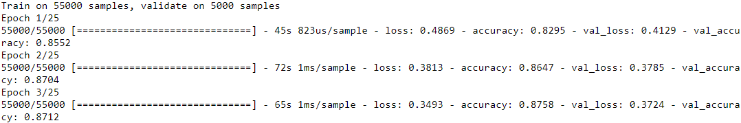
... ...
import matplotlib.pyplot as plt

learning_rate = 0.01
decay = 1e-4
batch_size=32
n_steps_per_epoch = len(X_train) //batch_size
epochs = np.arange(n_epochs)
lrs = learning_rate / (1 + decay* epochs*n_steps_per_epoch )

plt.plot( epochs, lrs, "o-")
plt.axis([0, n_epochs-1, 0, 0.01])
plt.xlabel("Epoch")
plt.ylabel("Learning Rate")
plt.title("Power Scheduling", fontsize=14)
plt.grid(True)
plt.show()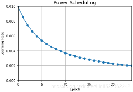
Exponential scheduling
- Set the learning rate to η(t) =
 OR
OR  . The learning rate will gradually drop by a factor of 10 every s OR r steps. While power scheduling reduces the learning rate more and more slowly, exponential scheduling keeps slashing大幅削减 it by a factor of 10 every s OR r steps.
@keras_export("keras.optimizers.schedules.ExponentialDecay")
class ExponentialDecay(LearningRateSchedule):
  """A LearningRateSchedule that uses an exponential decay schedule."""

  def __init__(
      self,
      initial_learning_rate,
      decay_steps,
      decay_rate,
      staircase=False,
      name=None):
    """Applies exponential decay to the learning rate.

    ```python
    def decayed_learning_rate(step):
      return initial_learning_rate * decay_rate ^ (step / decay_steps)
    ```

    ```python
    initial_learning_rate = 0.1
    lr_schedule = tf.keras.optimizers.schedules.ExponentialDecay(
        initial_learning_rate,
        decay_steps=100000,
        decay_rate=0.96,
        staircase=True)
    model.compile(optimizer=tf.keras.optimizers.SGD(learning_rate=lr_schedule),
                  loss='sparse_categorical_crossentropy',
                  metrics=['accuracy'])
    model.fit(data, labels, epochs=5)
    ```

    Args:
      initial_learning_rate: A scalar `float32` or `float64` `Tensor` or a
        Python number.  The initial learning rate.
      decay_steps: A scalar `int32` or `int64` `Tensor` or a Python number.
        Must be positive.  See the decay computation above.
      decay_rate: A scalar `float32` or `float64` `Tensor` or a
        Python number.  The decay rate.
      staircase: Boolean.  If `True` decay the learning rate at discrete
        intervals
      name: String.  Optional name of the operation.  Defaults to
        'ExponentialDecay'.

    """
    super(ExponentialDecay, self).__init__()
    self.initial_learning_rate = initial_learning_rate
    self.decay_steps = decay_steps
    self.decay_rate = decay_rate
    self.staircase = staircase
    self.name = name

  def __call__(self, step):
    with ops.name_scope_v2(self.name or "ExponentialDecay") as name:
      initial_learning_rate = ops.convert_to_tensor_v2(
          self.initial_learning_rate, name="initial_learning_rate")     # initial_learning_rate
      dtype = initial_learning_rate.dtype
      decay_steps = math_ops.cast(self.decay_steps, dtype)
      decay_rate = math_ops.cast(self.decay_rate, dtype)                # 0.1

      global_step_recomp = math_ops.cast(step, dtype)
      p = global_step_recomp / decay_steps                              # t/s=step /decay_steps
      if self.staircase:
        p = math_ops.floor(p)
      return math_ops.multiply(
          initial_learning_rate, math_ops.pow(decay_rate, p), name=name)#initial_learning_rate*decay_rate^(t/s)
lr = lr0 * 0.1**(epoch / s)
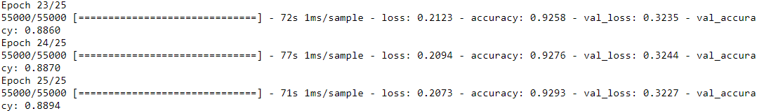
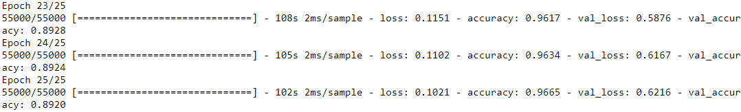
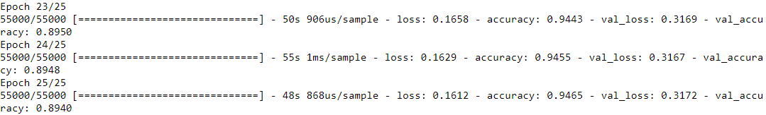
Exponential scheduling and piecewise scheduling are quite simple too. You first need to define a function that takes the current epoch and returns the learning rate. For example, let’s implement exponential scheduling:# initial_learning_rate = 0.01 # lr_schedule = tf.keras.optimizers.schedules.ExponentialDecay( # initial_learning_rate, # decay_steps=20, # decay_rate=0.1, # staircase=True # ) # You first need to define a function that takes the current epoch and returns the # learning rate. For example, let’s implement exponential scheduling: # def exponential_decay_fn(epoch): #epoch is global_step_recomp or step or 't' # return 0.01 * 0.1**(epoch/20) def exponential_decay(lr0, s): # def exponential_decay(lr0=0.01, s=20): def exponential_decay_fn(epoch): #epoch is global_step_recomp or step or 't' return lr0 * 0.1**(epoch/s) return exponential_decay_fn #不加括号就是返回函数对象,不是函数调用 exponential_decay_fn = exponential_decay(lr0=0.01, s=20) model = keras.models.Sequential([ keras.layers.Flatten( input_shape=[28,28]), keras.layers.Dense(300, activation="selu", kernel_initializer="lecun_normal"), keras.layers.Dense(100, activation="selu", kernel_initializer="lecun_normal"), keras.layers.Dense(10, activation="softmax") ]) model.compile( loss="sparse_categorical_crossentropy", optimizer="nadam", metrics=["accuracy"]) n_epochs = 25Next, create a LearningRateScheduler callback, giving it the schedule function, and pass this callback to the fit() method:
lr_scheduler = keras.callbacks.LearningRateScheduler( exponential_decay_fn )
history = model.fit(X_train_scaled, y_train, epochs=n_epochs,
                    validation_data=(X_valid_scaled, y_valid),
                    callbacks=[lr_scheduler])
The LearningRateScheduler will update the optimizer’s learning_rate attribute at the beginning of each epoch. Updating the learning rate once per epoch is usually enough, but if you want it to be updated more often, for example at every step, you can always write your own callback (see the “Exponential Scheduling” section of the notebook for an example). Updating the learning rate at every step makes sense if there are many steps per epoch. Alternatively, you can use the keras.optimizers.schedules approach, described shortly.
-
... ...
history.history.keys()
plt.plot(history.epoch, history.history["lr"], "o-")
plt.axis([0, n_epochs-1, 0, 0.011])
plt.xlabel("Epoch")
plt.ylabel("Learning Rate")
plt.title("Exponential Scheduling", fontsize=14)
plt.grid(True)
plt.show()
The schedule function can take the current learning rate as a second argument: For example, the following schedule function multiplies the previous learning rate by , which results in the same exponential decay (except the decay now starts at the beginning of epoch 0 instead of 1):
def exponential_decay_fn(epoch, current_lr):
    return current_lr*0.1**(1/20) #    decay_steps=20, decay_rate=0.1, steps=t=current epoch when ignoring epoch value
When you save a model, the optimizer and its learning rate get saved along with it. This means that with this new schedule function, you could just load a trained model and continue training where it left off, no problem. Things are not so simple if your schedule function uses the epoch argument, however: the epoch does not get saved, and it gets reset to 0 every time you call the fit() method. If you were to continue training a model where it left off, this could lead to a very large learning rate, which would likely damage your model’s weights. One solution is to manually set the fit() method’s initial_epoch argument so the epoch starts at the right value.
If you want to update the learning rate at each iteration rather than at each epoch(n_epochs=25), you must write your own callback class:
K = keras.backend

class ExponentialDecay( keras.callbacks.Callback ):
    def __init__(self, s=40000): #s: decay_steps
        super().__init__()
        self.s = s

    def on_batch_begin(self, batch, logs=None):
        ### Original
        ### batch: integer, index of batch within the current epoch. #each epoch has batch_size=32
        ### the learing rate is updated at each poch
        #now
        #  the learing rate is updated at each batch
        # Note: the `batch` argument is reset at each epoch
        lr = K.get_value(self.model.optimizer.lr)
        #print('\nbatch: ', batch, ' learing rate: ', lr,'\n')
        K.set_value(self.model.optimizer.lr, lr*0.1**(1/s)) #s: decay_steps #s = 20*len(X_train)//32

    def on_epoch_end( self, epoch, logs=None):
        logs = logs or {}
        logs['lr'] = K.get_value(self.model.optimizer.lr)

model = keras.models.Sequential([
    keras.layers.Flatten(input_shape=[28,28]),
    keras.layers.Dense(300, activation="selu", kernel_initializer="lecun_normal"),
    keras.layers.Dense(100, activation="selu", kernel_initializer="lecun_normal"),
    keras.layers.Dense(10, activation="softmax")
])

lr0=0.01
optimizer = keras.optimizers.Nadam(lr=lr0)
model.compile( loss="sparse_categorical_crossentropy", optimizer=optimizer, metrics=['accuracy'])
n_epochs=25

s = 20*len(X_train)//32  # number of steps in 20 epochs (batch size = 32)
exp_decay = ExponentialDecay(s)
history = model.fit(X_train_scaled, y_train, epochs=n_epochs,
                    validation_data = (X_valid_scaled, y_valid),
                    callbacks=[exp_decay])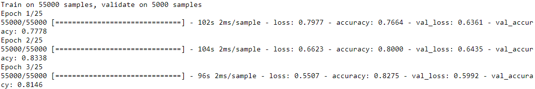
... ...
n_steps = n_epochs * len(X_train) //32 #n_epochs=25
steps = np.arange(n_steps)
lrs = lr0 * 0.1**(steps/s) #s = 20*len(X_train)//32

plt.plot(steps, lrs, "-", linewidth=2)
plt.axis([0, n_steps-1, 0, lr0 * 1.1])
plt.xlabel("Batch")
plt.ylabel("Learning Rate")
plt.title("Exponential Scheduling (per batch)", fontsize=14)
plt.grid(True)
plt.show()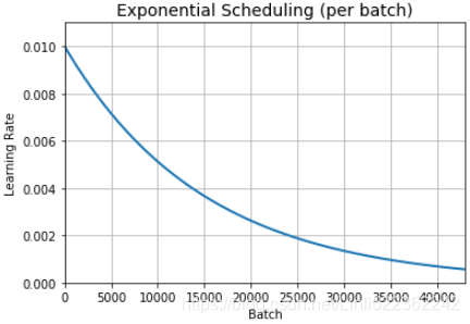
Piecewise constant scheduling分段恒定调度:
def fun(x): # 类似于 lambda(x):
    return x
fun(3) ![]()
等价于
fun=lambda x:x # 后面的x是返回语句
fun(3) ![]()
l= [lambda:n for n in range(5)]
for x in l:
print(x()) # each element in the list l is lambda statement, so we need to call with "()"![]()
和以下的形式应该等价:
l=[]
# lambda:n for n in range(5)
def fun():
    for n in range(5):
        n=n
    return n
for n in range(5): #since the lambda is in the list and call lambda statement 5 times
   l.append(fun) #append a function object to the list l
for x in l:
print(x())![]()
l= [lambda n=i:n for i in range(5)]#OR# l= [lambda n=n:n for n in range(5)]

for x in l:
print(x())![]()
l=[]
for i in range(5):
    def fun(n=i): #lambda n=i:n
        return n
    l.append(fun) #append a function object to the list

for x in l:
print(x()) ![]()
@keras_export("keras.optimizers.schedules.PiecewiseConstantDecay")
class PiecewiseConstantDecay(LearningRateSchedule):
  """A LearningRateSchedule that uses a piecewise constant decay schedule."""

  def __init__(
      self,
      boundaries,
      values,
      name=None):
    """Piecewise constant from boundaries and interval values.

    Example: use a learning rate that's
    1.0 for the first 100001 steps,
    0.5 for the next 10000 steps, and
    0.1 for any additional steps.
    ```python
    step = tf.Variable(0, trainable=False)
    boundaries = [100000, 110000]
    values = [1.0,     0.5,     0.1]
    learning_rate_fn = keras.optimizers.schedules.PiecewiseConstantDecay(
        boundaries, values)
    # Later, whenever we perform an optimization step, we pass in the step.
    learning_rate = learning_rate_fn(step)
    ```

    Args:
      boundaries: A list of `Tensor`s or `int`s or `float`s with strictly
        increasing entries, and with all elements having the same type as the
        optimizer step.
      values: A list of `Tensor`s or `float`s or `int`s that specifies the
        values for the intervals defined by `boundaries`. It should have one
        more element than `boundaries`, and all elements should have the same
        type.
      name: A string. Optional name of the operation. Defaults to
        'PiecewiseConstant'.
    Returns:
      The output of the 1-arg function that takes the `step`
      is `values[0]` when `step <= boundaries[0]`,
      `values[1]` when `step > boundaries[0]` and `step <= boundaries[1]`, ...,
      and values[-1] when `step > boundaries[-1]`.
    Raises:
      ValueError: if the number of elements in the lists do not match.
    """
    super(PiecewiseConstantDecay, self).__init__()

    if len(boundaries) != len(values) - 1:
      raise ValueError(
          "The length of boundaries should be 1 less than the length of values")

    self.boundaries = boundaries
    self.values = values
    self.name = name

  def __call__(self, step):
    with ops.name_scope_v2(self.name or "PiecewiseConstant"):
      boundaries = ops.convert_n_to_tensor(self.boundaries)
      values = ops.convert_n_to_tensor(self.values)
      x_recomp = ops.convert_to_tensor_v2(step)
      for i, b in enumerate(boundaries):
        if b.dtype.base_dtype != x_recomp.dtype.base_dtype:
          # We cast the boundaries to have the same type as the step
          b = math_ops.cast(b, x_recomp.dtype.base_dtype)
          boundaries[i] = b
      pred_fn_pairs = []
      pred_fn_pairs.append((x_recomp <= boundaries[0], lambda: values[0]))
      pred_fn_pairs.append((x_recomp > boundaries[-1], lambda: values[-1]))
      for low, high, v in zip(boundaries[:-1], boundaries[1:], values[1:-1]):
        # Need to bind v here; can do this with lambda v=v: ...
        pred = (x_recomp > low) & (x_recomp <= high)
        pred_fn_pairs.append((pred, lambda v=v: v))#中间的v是引用当前for中的v值,并保存
        ############################lambda(v=v): return v

      # The default isn't needed here because our conditions are mutually
      # exclusive and exhaustive, but tf.case requires it.
      default = lambda: values[0]
return control_flow_ops.case(pred_fn_pairs, default, exclusive=True)- Use a constant learning rate for a number of epochs (e.g.,
 = 0.1 for 5 epochs), then a smaller learning rate for another number of epochs (e.g.,
  = 0.001 for 50 epochs), and so on. Although this solution can work very well, it requires fiddling around摆弄 to figure out the right sequence of learning rates and how long to use each of them.
 def piecewise_constant_fn(epoch): if epoch < 5: return 0.01 elif epoch<15: return 0.005 else: return 0.001def piecewise_constant(boundaries, values): #values: learning rates boundaries = np.array( [0] + boundaries ) # array([0,5,15]) values = np.array(values) def piecewise_constant_fn(epoch): return values[ np.argmax(boundaries>epoch)-1 ]#np.argmax(boundaries>epoch) if boundaries>epoch then return its index return piecewise_constant_fn #return function object/ address piecewise_constant_fn = piecewise_constant([5,15], [0.01,0.005, 0.001]) lr_scheduler = keras.callbacks.LearningRateScheduler(piecewise_constant_fn) model = keras.models.Sequential([ keras.layers.Flatten( input_shape=[28,28] ), keras.layers.Dense(300, activation="selu", kernel_initializer="lecun_normal"), keras.layers.Dense(100, activation="selu", kernel_initializer="lecun_normal"), keras.layers.Dense(10, activation="softmax") ]) model.compile( loss="sparse_categorical_crossentropy", optimizer="nadam", metrics=['accuracy']) n_epochs=25 history=model.fit(X_train_scaled, y_train, epochs=n_epochs, validation_data=(X_valid_scaled, y_valid), callbacks=[lr_scheduler])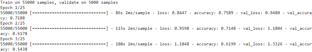
... ...
plt.plot(history.epoch, [piecewise_constant_fn(epoch) for epoch in history.epoch], "o-")
plt.axis([0, n_epochs-1, 0, 0.011])
plt.xlabel("Epoch")
plt.ylabel("Learning Rate")
plt.title("Piecewise Constant Scheduling", fontsize=14)
plt.grid(True)
plt.show()
Performance Scheduling
- Measure the validation error every N steps (just like for early stopping), and reduce the learning rate by a factor of λ when the error stops dropping.
For performance scheduling, use the ReduceLROnPlateau callback. For example, if you pass the following callback to the fit() method, it will multiply the learning rate by 0.5 whenever the best validation loss does not improve for five consecutive epochs (other options are available; please check the documentation for more details):tf.random.set_seed(42) np.random.seed(42) # factor: factor by which the learning rate will be reduced. new_lr = lr * factor # patience: number of epochs with no improvement after which learning rate will be reduced. lr_scheduler = keras.callbacks.ReduceLROnPlateau(factor=0.5, patience=5) model = keras.models.Sequential([ keras.layers.Flatten( input_shape=[28,28] ), keras.layers.Dense( 300, activation="selu", kernel_initializer="lecun_normal" ), keras.layers.Dense( 100, activation="selu", kernel_initializer="lecun_normal" ), keras.layers.Dense( 10, activation="softmax") ]) optimizer = keras.optimizers.SGD( lr=0.02, momentum=0.9 ) model.compile( loss="sparse_categorical_crossentropy", optimizer=optimizer, metrics=['accuracy']) n_epochs = 25 history = model.fit( X_train_scaled, y_train, epochs=n_epochs, validation_data=(X_valid_scaled, y_valid), callbacks = [lr_scheduler])
... ...
plt.plot(history.epoch, history.history['lr'], "bo-")
plt.xlabel("Epoch")
plt.ylabel("Learning Rate", color="b")
plt.tick_params('y', colors="b")
plt.gca().set_xlim(0, n_epochs-1)
plt.grid(True)

ax2 = plt.gca().twinx()
ax2.plot(history.epoch, history.history['val_loss'], "r^-")
ax2.set_ylabel("Validation Loss", color='r')
ax2.tick_params('y', color='r')

plt.title("Reduce LR on Plateau", fontsize=14)
plt.show()
Measure the validation error every N steps (just like for early stopping), and reduce the learning rate by a factor of λ when the error stops dropping.
 -
Lastly, tf.keras offers an alternative way to implement learning rate scheduling: define the learning rate using one of the schedules available in keras.optimizers.schedules, then pass this learning rate to any optimizer. This approach updates the learning rate at each step rather than at each epoch.
For example, here is how to implement
the same exponential schedule as the exponential_decay_fn() function we defined earlier:model = keras.models.Sequential([ keras.layers.Flatten( input_shape=[28,28]), keras.layers.Dense(300, activation="selu", kernel_initializer="lecun_normal"), keras.layers.Dense(100, activation="selu", kernel_initializer="lecun_normal"), keras.layers.Dense(10, activation="softmax") ]) s= 20*len(X_train)//32 # number of steps in 20 epochs (batch size = 32) #decay_steps # ExponentialDecay( initial_learning_rate, decay_steps, decay_rate, staircase=False, name=None ) # The learning rate will gradually drop by a factor of 100 every s OR r decay_steps. learning_rate = keras.optimizers.schedules.ExponentialDecay(0.01, s, 0.1) optimizer = keras.optimizers.SGD( learning_rate ) model.compile(loss="sparse_categorical_crossentropy", optimizer=optimizer, metrics=['accuracy']) n_epochs = 25 history = model.fit(X_train_scaled, y_train, epochs=n_epochs, validation_data=(X_valid_scaled, y_valid))This is nice and simple, plus when you save the model, the learning rate and its
schedule (including its state) get saved as well. This approach, however, is not part of
the Keras API; it is specific to tf.keras.
... ...
For piecewise constant scheduling, try this:learning_rate = keras.optimizers.schedules.PiecewiseConstantDecay( boundaries=[5. * n_steps_per_epoch, 15. * n_steps_per_epoch], values=[0.01, 0.005, 0.001])
1cycle scheduling
Contrary to the other approaches, 1cycle (introduced in a 2018 paper by Leslie Smith) starts by increasing the initial learning rate ![]() , growing linearly up to
, growing linearly up to ![]() halfway through training. Then it decreases the learning rate linearly down to
halfway through training. Then it decreases the learning rate linearly down to ![]() again during the second half of training, finishing the last few epochs by dropping the rate down by several orders of magnitude (still linearly). The maximum learning rate
again during the second half of training, finishing the last few epochs by dropping the rate down by several orders of magnitude (still linearly). The maximum learning rate ![]() is chosen using the same approach we used to find the optimal learning rate, and the initial learning rate
is chosen using the same approach we used to find the optimal learning rate, and the initial learning rate ![]() is chosen to be roughly 10 times lower. When using a momentum, we start with a high momentum first (e.g., 0.95), then drop it down to a lower momentum during the first half of training (e.g., down to 0.85, linearly), and then bring it back up to the maximum value (e.g., 0.95) during the second half of training, finishing the last few epochs with that maximum value. Smith did many experiments showing that this approach was often able to speed up training considerably and reach better performance. For example, on the popular CIFAR10 image dataset, this approach reached 91.9% validation accuracy in just 100 epochs, instead of 90.3% accuracy in 800 epochs through a standard approach (with the same neural network architecture).
is chosen to be roughly 10 times lower. When using a momentum, we start with a high momentum first (e.g., 0.95), then drop it down to a lower momentum during the first half of training (e.g., down to 0.85, linearly), and then bring it back up to the maximum value (e.g., 0.95) during the second half of training, finishing the last few epochs with that maximum value. Smith did many experiments showing that this approach was often able to speed up training considerably and reach better performance. For example, on the popular CIFAR10 image dataset, this approach reached 91.9% validation accuracy in just 100 epochs, instead of 90.3% accuracy in 800 epochs through a standard approach (with the same neural network architecture).

K = keras.backend

class ExponentialLearningRate( keras.callbacks.Callback):
    def __init__(self, factor):
        self.factor = factor
        self.rates = []
        self.losses = []

    def on_batch_end(self, batch, logs):# from keras.callbacks.Callback
        self.rates.append( K.get_value(self.model.optimizer.lr) )
        self.losses.append( logs['loss'] )
        K.set_value( self.model.optimizer.lr, self.model.optimizer.lr*self.factor )#update learning rate#callback

def find_learing_rate( model, X,y, epochs=1, batch_size=32, min_rate=10**-5, max_rate=10):
    init_weights = model.get_weights()

    iterations = len(X) // batch_size * epochs
    factor = np.exp(np.log(max_rate / min_rate)/iterations)
    init_lr = K.get_value(model.optimizer.lr)   # get initial learning rate
    K.set_value( model.optimizer.lr, min_rate ) # replace initial learning rate with min_rate
    exp_lr = ExponentialLearningRate(factor)    # pass learning rate factor to
    history = model.fit( X, y, epochs=epochs, batch_size=batch_size, callbacks=[exp_lr] )
    K.set_value( model.optimizer.lr, init_lr )  # replace current learning rate with initiallearning rate

    model.set_weights(init_weights)
    return exp_lr.rates, exp_lr.losses

def plot_lr_vs_loss( rates, losses ):
    plt.plot(rates, losses)
    plt.gca().set_xscale("log")
    plt.hlines( min(losses), min(rates),max(rates) )
    plt.axis( [min(rates), max(rates),  min(losses), (losses[0]+min(losses))/2 ])
    plt.xlabel("Learning rate")
    plt.ylabel("Loss")
tf.random.set_seed(42)
np.random.seed(42)
model = keras.models.Sequential([
keras.layers.Flatten(input_shape=[28,28]),
keras.layers.Dense(300, activation="selu", kernel_initializer="lecun_normal"),
keras.layers.Dense(100, activation="selu", kernel_initializer="lecun_normal"),
keras.layers.Dense(10, activation="softmax")
])
model.compile( loss="sparse_categorical_crossentropy",
optimizer=keras.optimizers.SGD(lr=1e-3),
metrics=["accuracy"])
batch_size=128
rates, losses = find_learing_rate( model, X_train_scaled, y_train, epochs=1, batch_size=batch_size)
plot_lr_vs_loss(rates, losses)
To sum up, exponential decay, performance scheduling, and 1cycle can considerably speed up convergence, so give them a try!
class OneCycleScheduler( keras.callbacks.Callback ):
    def __init__(self, iterations, max_rate, start_rate=None,
                 last_iterations=None, last_rate=None):

        self.iterations = iterations #total iterations

        self.max_rate = max_rate
        self.start_rate = start_rate or max_rate/10

        self.last_iterations = last_iterations or iterations//10+1
        self.half_iteration_pos = (iterations - self.last_iterations)//2

        # finishing the last few epochs by dropping the rate down by several orders of magnitude
        self.last_rate = last_rate or self.start_rate/1000

        self.iteration_pos = 0

    def _iterpolate( self, iter1, iter2,
                           rate1, rate2):
                 # a_slope: (rate2-rate1)/(iter2-iter1)
                 # x: (self.iteration-iter1)
                 # b: rate1
                 # y= a_slope * x + b
        return ( (rate2-rate1)*(self.iteration_pos-iter1) / (iter2-iter1) + rate1 )

    def on_batch_begin(self, batch, logs):
        if self.iteration_pos < self.half_iteration_pos:
            rate = self._iterpolate(0, self.half_iteration_pos,
                                    self.start_rate, self.max_rate)

        elif self.iteration_pos < 2*self.half_iteration_pos:
            rate = self._iterpolate(self.half_iteration_pos, 2*self.half_iteration_pos,
                                    self.max_rate, self.start_rate)
        else:
            rate = self._iterpolate(2*self.half_iteration_pos, self.iterations,
                                    self.start_rate, self.last_rate)
        self.iteration_pos +=1
        K.set_value(self.model.optimizer.lr, rate)#update
n_epochs = 25 #note each batch tacks n_epochs
onecycle = OneCycleScheduler( len(X_train)//batch_size * n_epochs, max_rate=0.05) #max_rate=0.05 and loss=1.0
history = model.fit(X_train_scaled, y_train, epochs=n_epochs, batch_size=batch_size,
validation_data=(X_valid_scaled, y_valid),
callbacks=[onecycle])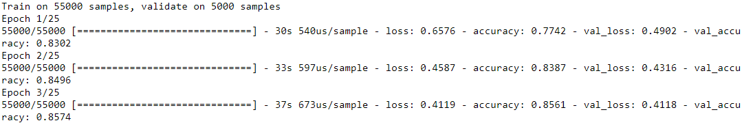
... ...
A 2013 paper by Andrew Senior et al. compared the performance of some of the most popular learning schedules when using momentum optimization to train deep neural networks for speech recognition. The authors concluded that, in this setting,
both performance scheduling and exponential scheduling performed well. They favored exponential scheduling because it was easy to tune and it converged slightly faster to the optimal solution (they also mentioned that it was easier to implement than performance scheduling, but in Keras both options are easy). That said, the 1cycle approach seems to perform even better.
Avoiding Overfitting Through Regularization
With thousands of parameters, you can fit the whole zoo. Deep neural networks typically have tens of thousands of parameters, sometimes even millions. This gives them an incredible amount of freedom and means they can fit a huge variety of complex datasets. But this great flexibility also makes the network prone to overfitting the training set. We need regularization.
We already implemented one of the best regularization techniques in Chapter 10: early stopping (cp4:https://blog.csdn.net/Linli522362242/article/details/104124771, cp10: https://blog.csdn.net/Linli522362242/article/details/106582512). Moreover, even though Batch Normalization was designed to solve the unstable gradients problems, it also acts like a pretty good regularizer. In this section we will examine other popular regularization techniques for neural networks: ℓ1 and ℓ2 regularization, dropout, and max-norm regularization.
 and
and  Regularization
Just like you did in Chapter 4 for simple linear models(https://blog.csdn.net/Linli522362242/article/details/104070847), you can use ![]() regularization to constrain a neural network’s connection weights, and/or
regularization to constrain a neural network’s connection weights, and/or ![]() regularization if you want a sparse model (with many weights equal to 0).
regularization if you want a sparse model (with many weights equal to 0).
Here is how to apply ![]() regularization to a Keras layer’s connection weights, using a regularization factor of 0.01:
regularization to a Keras layer’s connection weights, using a regularization factor of 0.01:
from tensorflow import keras

layer = keras.layers.Dense(100, activation="elu", kernel_initializer = "he_normal",
                           kernel_regularizer = keras.regularizers.l2(0.01))
# or l1(0.1) for ℓ1 regularization with a factor or 0.1
# or l1_l2(0.1, 0.01) for both ℓ1 and ℓ2 regularization, with factors 0.1 and 0.01 respectively
The l2() function returns a regularizer that will be called at each step during training to compute the regularization loss. This is then added to the final loss. As you might expect, you can just use keras.regularizers.l1() if you want ℓ1 regularization; if
you want both ℓ1 and ℓ2 regularization, use keras.regularizers.l1_l2() (specifying both regularization factors).
model = keras.models.Sequential([
keras.layers.Flatten(input_shape=[28,28]), #exponential linear unit (ELU)
keras.layers.Dense( 300, activation="elu", kernel_regularizer=keras.regularizers.l2(0.01) ),
keras.layers.Dense( 100, activation="elu", kernel_regularizer=keras.regularizers.l2(0.01) ),
keras.layers.Dense( 10, activation="softmax", kernel_regularizer=keras.regularizers.l2(0.01) )
])
model.compile(loss="sparse_categorical_crossentropy", optimizer="nadam", metrics=["accuracy"])
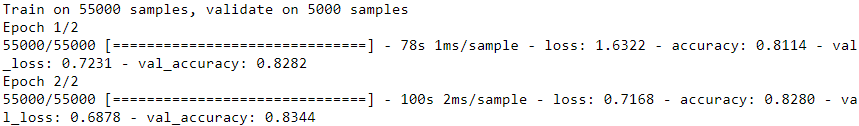
n_epochs=2
history = model.fit(X_train_scaled, y_train, epochs=n_epochs,
validation_data = (X_valid_scaled, y_valid))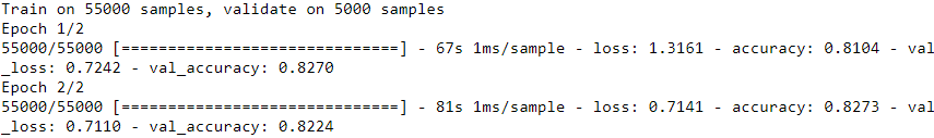
l2(0.01) means every coefficient in the weight matrix of the layer will add 0.01* weight_coefficient_value to the total loss of the network. Note that because this penalty is only added at training time, the loss for this network will be much higher at training than at test time.
Since you will typically want to apply the same regularizer to all layers in your network, as well as using the same activation function and the same initialization strategy in all hidden layers, you may find yourself repeating the same arguments. This makes the code ugly丑陋 and error-prone. To avoid this, you can try refactoring your code to use loops. Another option is to use Python’s functools.partial() function, which lets you create a thin wrapper for any callable, with some default argument values:
from functools import partial

RegularizedDense = partial( keras.layers.Dense,
                            activation="elu",
                            kernel_initializer = "he_normal",
                            kernel_regularizer = keras.regularizers.l2(0.01)
                          )

model = keras.Sequential([
    keras.layers.Flatten( input_shape=[28,28]),
    RegularizedDense(300),
    RegularizedDense(100),
    RegularizedDense(10, activation="softmax")
])
model.compile(loss="sparse_categorical_crossentropy", optimizer="nadam", metrics=["accuracy"])
n_epochs = 2
history = model.fit(X_train_scaled, y_train, epochs = n_epochs,
                    validation_data=(X_valid_scaled, y_valid))
Dropout
https://blog.csdn.net/Linli522362242/article/details/107164478