Python数据分析与机器学习----收入的预测分析

一、题目

利用age、workclass、…、native_country等13个特征预测收入是否超过50k，是一个二分类问题。

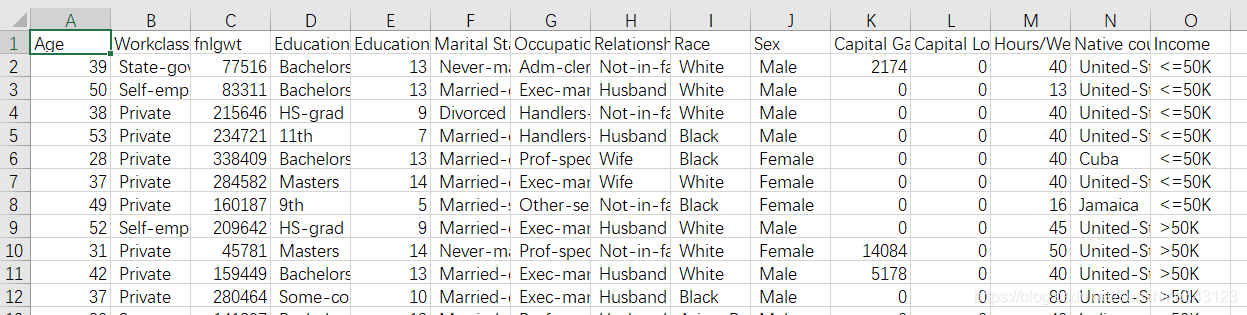
二、训练集

32561个样本，每个样本14个特征，其中6个连续性特征、9个离散型特征

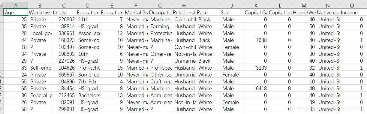
三、测试集

16281个样本，每个样本14个特征，
即在测试集中，根据age等14个特征，预测income是否超过50k，二分类问题。

四、说明

部分特征的值为“？”，表示缺失值，需要对其先处理。

五、实验过程和结果

import numpy as np
import pandas as pd
train = pd.read_csv('data/data40587/train.csv')
train.replace(' ?', np.nan, inplace=True)
print(train.isnull().sum())

#用众数进行替换缺失值
train.fillna(value = {
    
    'Workclass':train.Workclass.mode()[0],
                              'Occupation':train.Occupation.mode()[0],
                              'Native country':train['Native country'].mode()[0]}, inplace = True)

# 数据的探索性分析、数值型的统计描述
print(train.describe())
# 数据的探索性分析、离散型的统计描述
print(train.describe(include =[ 'object']))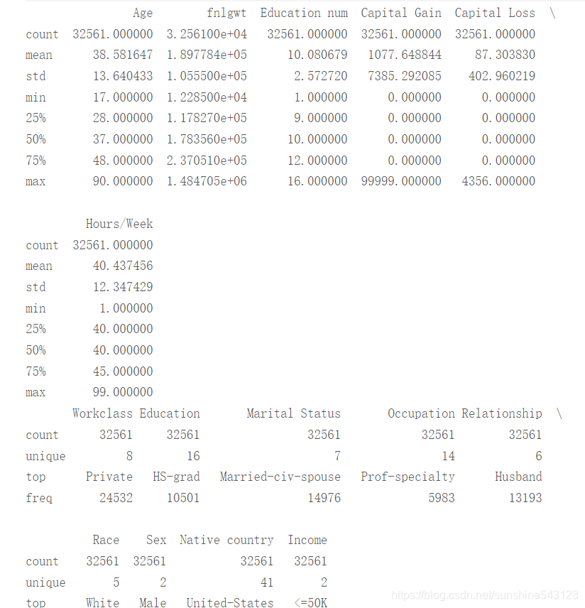

# 导入绘图模块
import matplotlib.pyplot as plt
# 设置绘图风格
plt.style.use('ggplot')
# 设置多图形的组合
fig, axes = plt.subplots(2, 1)
# 绘制不同收入水平下的年龄核密度图，    针对数值型
train['Age'][train.Income == ' <=50K'].plot(kind = 'kde', label = '<=50K', ax = axes[0], legend = True, linestyle = '-')
train['Age'][train.Income == ' >50K'].plot(kind = 'kde', label = '>50K', ax = axes[0], legend = True, linestyle = '--')
# 绘制不同收入水平下的周工作小时数和密度图
train['Hours/Week'][train.Income == ' <=50K'].plot(kind = 'kde', label = '<=50K', ax = axes[1], legend = True, linestyle = '-')
train['Hours/Week'][train.Income == ' >50K'].plot(kind = 'kde', label = '>50K', ax = axes[1], legend = True, linestyle = '--')
# 显示图形
plt.show()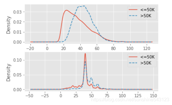

import seaborn as sns
# 构造不同收入水平下各种族人数的数据    针对离散型
race = pd.DataFrame(train.groupby(by = ['Race','Income']).aggregate(np.size).loc[:,'Age'])
# 重设行索引
race = race.reset_index()
# 变量重命名
race.rename(columns={
    
    'Age':'counts'}, inplace=True)
# 排序
race.sort_values(by = ['Race','counts'], ascending=False, inplace=True)

# 构造不同收入水平下各家庭关系人数的数据
relationship = pd.DataFrame(train.groupby(by = ['Relationship','Income']).aggregate(np.size).loc[:,'Age'])
relationship = relationship.reset_index()
relationship.rename(columns={
    
    'Age':'counts'}, inplace=True)
relationship.sort_values(by = ['Relationship','counts'], ascending=False, inplace=True)

# 设置图框比例，并绘图
plt.figure(figsize=(9,5))
sns.barplot(x="Race", y="counts", hue = 'Income', data=race)
plt.show()

plt.figure(figsize=(9,5))
sns.barplot(x="Relationship", y="counts", hue = 'Income', data=relationship)
plt.show()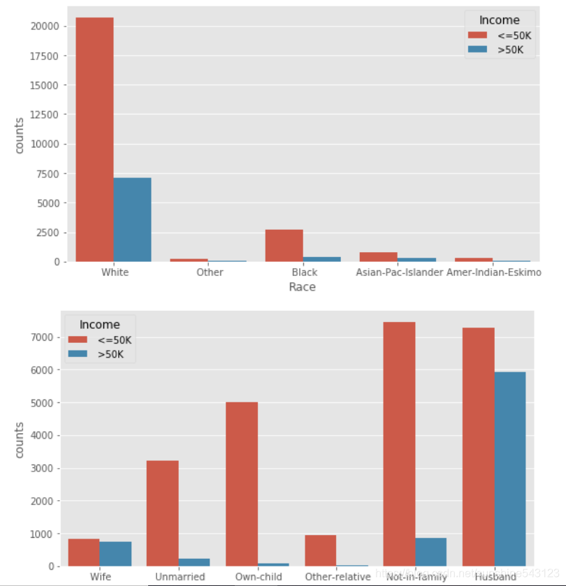

# 离散变量的重编码
for feature in train.columns:
    if train[feature].dtype == 'object':
        train[feature] = pd.Categorical(train[feature]).codes
print(train.head())
# 删除变量
train.drop(['Education','fnlgwt'], axis = 1, inplace = True)
#训练集拆分
train_arr=np.array(train) #转换为数组
X_train=np.delete(train_arr,12,axis=1)
i_=[0,1,2,3,4,5,6,7,8,9,10,11]
y_train=np.delete(train_arr,i_,axis=1)

# 导入k近邻模型的类
from sklearn.neighbors import KNeighborsClassifier
# 构建k近邻模型
kn = KNeighborsClassifier()
kn.fit(X_train, y_train)
print(kn)

#整理测试数据集

# 加载测试数据集
test = pd.read_csv('data/data40587/test.csv')
test.replace(' ?', np.nan, inplace=True)
print(test.isnull().sum())
#用众数进行替换缺失值
test.fillna(value = {
    
    'Workclass':test.Workclass.mode()[0],
                              'Occupation':test.Occupation.mode()[0],
                              'Native country':test['Native country'].mode()[0]}, inplace = True)
# 离散变量的重编码
for feature in test.columns:
    if test[feature].dtype == 'object':
        test[feature] = pd.Categorical(test[feature]).codes

# 删除变量
test.drop(['Education','fnlgwt'], axis = 1, inplace = True)
print(test.head())

# 预测测试集
kn_pred = kn.predict(test)
#保存结果
test1 = pd.read_csv('data/data40587/test.csv')
test1['Income'] =kn_pred
test1.to_csv("20200618.csv",index=None)

结果