tf.keras快速入门——函数式API

在上篇中简单的使用了序列模型，由于序列模型只能表示为神经网络层的简单堆叠，而无法表示成任意模型。故而这里将使用函数式API来构建更加复杂的模型。
在鸢尾花分类一文中简单使用了序列模型来解决这个问题，这里将使用函数式API来解决这个问题，体验使用函数式API的便捷性。
先看看官方案例：

import tensorflow as tf

inputs = tf.keras.Input(shape=(3,))
x = tf.keras.layers.Dense(4, activation=tf.nn.relu)(inputs)
outputs = tf.keras.layers.Dense(5, activation=tf.nn.softmax)(x)
model = tf.keras.Model(inputs=inputs, outputs=outputs)

修改后的代码如下：

import matplotlib.pyplot as plt
%matplotlib inline
import tensorflow as tf
from sklearn.datasets import load_iris
# 训练集和测试集的划分
from sklearn.model_selection import train_test_split

x_data = load_iris().data  # 特征，【花萼长度,花萼宽度,花瓣长度,花瓣宽度】
y_data = load_iris().target # 分类
x_train, x_test, y_train, y_test = train_test_split(x_data, y_data, test_size=0.30, random_state=42)

input_data = tf.keras.Input(shape=(len(x_data[0],)))
h_1 = tf.keras.layers.Dense(4, activation="relu")(input_data)
h_2 = tf.keras.layers.Dense(3, activation="softmax")(h_1)

model = tf.keras.Model(inputs=input_data, outputs=h_2)
      
model.compile(optimizer=tf.keras.optimizers.Adam(), 
             loss=tf.keras.losses.sparse_categorical_crossentropy, 
             metrics=['accuracy'])

history = model.fit(x_train, y_train, epochs=300)


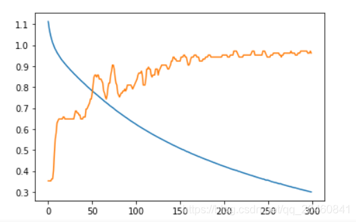
for key in history.history.keys():
    plt.plot(history.epoch, history.history[key])

其实，我们可以看见，在上面的小案例中，和鸢尾花分类一文中不同之处就在于可以任意指定神经网络层是和那一层相连的，然后加入了tf.keras.Input层。

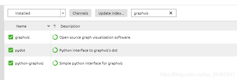
最后，不放看看网络的样子，首先我们需要安装pydot，graphviz和python-graphviz即可。
在Anaconda中的Navigator中直接搜索安装即可。

然后我们使用：

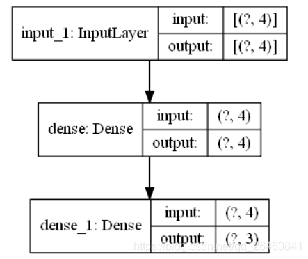
tf.keras.utils.plot_model(model, 'model_info.png', show_shapes=True)

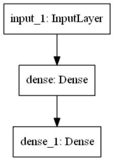
tf.keras.utils.plot_model(model, 'mnist_model.png')