文章目录
numpy & pandas
why numpy & pandas
- 运算速度快:numpy 和 pandas 都是采用 C 语言编写, pandas 又是基于 numpy, 是 numpy 的升级版本。
- 消耗资源少:采用的是矩阵运算,会比 python 自带的字典或者列表快好多
import numpy as np
numpy
属性
ndim:维度shape:行数和列数size:元素个数
列表转化为矩阵:
array = np.array([[1,2,3],[2,3,4]])  #列表转化为矩阵
print(array)
"""
array([[1, 2, 3],
       [2, 3, 4]])
"""
接着我们看看这几种属性的结果:
print('number of dim:',array.ndim)  # 维度
# number of dim: 2

print('shape :',array.shape)    # 行数和列数
# shape : (2, 3)

print('size:',array.size)   # 元素个数
# size: 6
numpy.array
https://numpy.org/doc/1.18/reference/generated/numpy.array.html?highlight=array#numpy.array
下面为例子
a = np.array([[2,23,4],[2,32,4]])  # 2d 矩阵 2行3列
print(a)
"""
[[ 2 23  4]
 [ 2 32  4]]
"""
创建全零数组
a = np.zeros((3,4)) # 数据全为0,3行4列
"""
array([[ 0.,  0.,  0.,  0.],
       [ 0.,  0.,  0.,  0.],
       [ 0.,  0.,  0.,  0.]])
"""
创建全一数组, 同时也能指定这些特定数据的 dtype:
a = np.ones((3,4),dtype = np.int)   # 数据为1,3行4列
"""
array([[1, 1, 1, 1],
       [1, 1, 1, 1],
       [1, 1, 1, 1]])
"""
创建全空数组, 其实每个值都是接近于零的数:
a = np.empty((3,4)) # 数据为empty,3行4列
"""
array([[  0.00000000e+000,   4.94065646e-324,   9.88131292e-324,
          1.48219694e-323],
       [  1.97626258e-323,   2.47032823e-323,   2.96439388e-323,
          3.45845952e-323],
       [  3.95252517e-323,   4.44659081e-323,   4.94065646e-323,
          5.43472210e-323]])
"""
用 arange 创建连续数组:
a = np.arange(10,20,2) # 10-19 的数据,2步长
"""
array([10, 12, 14, 16, 18])
"""
用 linspace 创建线段型数据:
a = np.linspace(1,10,20)    # 开始端1,结束端10,且分割成20个数据,生成线段
"""
array([  1.        ,   1.47368421,   1.94736842,   2.42105263,
         2.89473684,   3.36842105,   3.84210526,   4.31578947,
         4.78947368,   5.26315789,   5.73684211,   6.21052632,
         6.68421053,   7.15789474,   7.63157895,   8.10526316,
         8.57894737,   9.05263158,   9.52631579,  10.        ])
"""
numpy.reshape
https://numpy.org/doc/1.18/reference/generated/numpy.reshape.html?highlight=reshape#numpy.reshape
>>> a = np.arange(6).reshape((3, 2))
>>> a
array([[0, 1],
       [2, 3],
       [4, 5]])
基础运算
一维
让我们从一个脚本开始了解相应的计算以及表示形式 :
import numpy as np
a=np.array([10,20,30,40])   # array([10, 20, 30, 40])
b=np.arange(4)              # array([0, 1, 2, 3])

# 减法
c=a-b  # array([10, 19, 28, 37])

# 加法
c=a+b   # array([10, 21, 32, 43])

# 乘法
c=a*b   # array([  0,  20,  60, 120])

# 乘方
c=b**2  # array([0, 1, 4, 9])

# 三角函数
c=np.sin(a)
# array([-0.54402111  0.91294525 -0.98803162  0.74511316])
除了函数应用外,在脚本中对print函数进行一些修改可以进行逻辑判断:
print(b<3)
# [ True  True  True False]

print(b==2)
# [False False  True False]
二维或多维
上述运算均是建立在一维矩阵,即只有一行的矩阵上面的计算,如果我们想要对多行多维度的矩阵进行操作,需要对开始的脚本进行一些修改:
a=np.array([[1,1],[0,1]])
b=np.arange(4).reshape((2,2))

print(a)
# array([[1, 1],
#       [0, 1]])

print(b)
# array([[0, 1],
#       [2, 3]])
# 乘法

# 逐个相乘
c = a*b

#矩阵相乘
c_dot = np.dot(a,b)
# array([[2, 4],
#       [2, 3]])

# 矩阵相乘另一种表示
c_dot_2 = a.dot(b)
# array([[2, 4],
#       [2, 3]])
下面我们将重新定义一个脚本, 来看看关于 sum(), min(), max()的使用:
import numpy as np
a=np.random.random((2,4))
print(a)
# array([[ 0.94692159,  0.20821798,  0.35339414,  0.2805278 ],
#       [ 0.04836775,  0.04023552,  0.44091941,  0.21665268]])

# 在整个矩阵中查找/求和
np.sum(a)   # 4.4043622002745959
np.min(a)   # 0.23651223533671784
np.max(a)   # 0.90438450240606416

# 以行或列作为查找单位
# 当axis的值为0的时候,将会以列作为查找单元
# 当axis的值为1的时候,将会以行作为查找单元
np.sum(a, axis=1)	# sum = [ 1.96877324  2.43558896]
np.min(a, axis=0)	# min = [ 0.23651224  0.41900661  0.36603285  0.46456022]
np.max(a, axis=1)	# max = [ 0.84869417  0.9043845 ]
然而在日常使用中,对应元素的索引也是非常重要的。依然,让我们先从一个脚本开始 :
import numpy as np
A = np.arange(2,14).reshape((3,4))

# array([[ 2, 3, 4, 5]
#        [ 6, 7, 8, 9]
#        [10,11,12,13]])

# 求矩阵中最小元素和最大元素的索引
print(np.argmin(A))    # 0
print(np.argmax(A))    # 11

# 均值
print(np.mean(A))        # 7.5
print(A.mean())          # 7.5
print(np.average(A))     # 7.5

# 中位数
print(A.median())        # 7.5

# 累加
print(np.cumsum(A)) 	 # [2 5 9 14 20 27 35 44 54 65 77 90]

# 累差
print(np.diff(A))
# [[1 1 1]
#  [1 1 1]
#  [1 1 1]]

# 找出非0的数
print(np.nonzero(A))
# (array([0,0,0,0,1,1,1,1,2,2,2,2]),array([0,1,2,3,0,1,2,3,0,1,2,3]))
# 左边为行数,右边为列数
同样的,我们可以对所有元素进行仿照列表一样的排序操作,但这里的排序函数仍然仅针对每一行进行从小到大排序操作:
import numpy as np
A = np.arange(14, 2, -1).reshape((3,4))

# array([[14, 13, 12, 11],
#       [10,  9,  8,  7],
#       [ 6,  5,  4,  3]])

print(np.sort(A))

# array([[11,12,13,14]
#        [ 7, 8, 9,10]
#        [ 3, 4, 5, 6]])
矩阵的转置有两种表示方法:
print(np.transpose(A))
print(A.T)

# array([[14,10, 6]
#        [13, 9, 5]
#        [12, 8, 4]
#        [11, 7, 3]])
# array([[14,10, 6]
#        [13, 9, 5]
#        [12, 8, 4]
#        [11, 7, 3]])
特别的,在Numpy中具有clip()函数,例子如下:
print(A)
# array([[14,13,12,11]
#        [10, 9, 8, 7]
#        [ 6, 5, 4, 3]])

print(np.clip(A,5,9))
# array([[ 9, 9, 9, 9]
#        [ 9, 9, 8, 7]
#        [ 6, 5, 5, 5]])
这个函数的格式是clip(Array,Array_min,Array_max),顾名思义,Array指的是将要被执行用的矩阵,而后面的最小值最大值则用于让函数判断矩阵中元素是否有比最小值小的或者比最大值大的元素,并将这些指定的元素转换为最小值或者最大值。
索引
我们都知道,在元素列表或者数组中,我们可以用如同a[2]一样的表示方法,同样的,在Numpy中也有相对应的表示方法:
import numpy as np
A = np.arange(3,15)

# array([3, 4, 5, 6, 7, 8, 9, 10, 11, 12, 13, 14])

print(A[3])    # 6
让我们将矩阵转换为二维的,此时进行同样的操作:
A = np.arange(3,15).reshape((3,4))
"""
array([[ 3,  4,  5,  6]
       [ 7,  8,  9, 10]
       [11, 12, 13, 14]])
"""

print(A[2])
# [11 12 13 14]
实际上这时的A[2]对应的就是矩阵A中第三行(从0开始算第一行)的所有元素。
如果你想要表示具体的单个元素,可以仿照上述的例子:
print(A[1][1])      # 8

print(A[1, 1])      # 8
在Python的 list 中,我们可以利用:对一定范围内的元素进行切片操作,在Numpy中我们依然可以给出相应的方法:
print(A[1, 1:3]) # [8 9]
这一表示形式即针对第二行中第2到第4列元素进行切片输出(不包含第4列)。 此时我们适当的利用for函数进行打印:
for row in A:
    print(row)
"""
[ 3,  4,  5, 6]
[ 7,  8,  9, 10]
[11, 12, 13, 14]
"""
此时它会逐行进行打印操作。如果想进行逐列打印,就需要稍稍变化一下:
for column in A.T:
    print(column)
"""
[ 3,  7,  11]
[ 4,  8,  12]
[ 5,  9,  13]
[ 6, 10,  14]
"""
上述表示方法即对A进行转置,再将得到的矩阵逐行输出即可得到原矩阵的逐列输出。
最后依然说一些关于迭代输出的问题:
import numpy as np
A = np.arange(3,15).reshape((3,4))

print(A.flatten())
# array([3, 4, 5, 6, 7, 8, 9, 10, 11, 12, 13, 14])

for item in A.flat:
    print(item)

# 3
# 4
……
# 14
这一脚本中的flatten是一个展开性质的函数,将多维的矩阵进行展开成1行的数列。而flat是一个迭代器,本身是一个object属性。
array合并
np.vstack()
对于一个array的合并,我们可以想到按行、按列等多种方式进行合并。首先先看一个例子:
import numpy as np
A = np.array([1,1,1])
B = np.array([2,2,2])

print(np.vstack((A,B)))    # vertical stack
"""
[[1,1,1]
 [2,2,2]]
"""
vertical stack本身属于一种上下合并,即对括号中的两个整体进行对应操作。此时我们对组合而成的矩阵进行属性探究:
C = np.vstack((A,B))
print(A.shape,C.shape)

# (3,) (2,3)
np.hstack()
利用shape函数可以让我们很容易地知道A和C的属性,从打印出的结果来看,A仅仅是一个拥有3项元素的数组(数列),而合并后得到的C是一个2行3列的矩阵。
介绍完了上下合并,我们来说说左右合并:
D = np.hstack((A,B))       # horizontal stack

print(D)
# [1,1,1,2,2,2]

print(A.shape,D.shape)
# (3,) (6,)
通过打印出的结果可以看出:D本身来源于A,B两个数列的左右合并,而且新生成的D本身也是一个含有6项元素的序列。
np.newaxis()
说完了array的合并,我们稍稍提及一下前一节中转置操作,如果面对如同前文所述的A序列, 转置操作便很有可能无法对其进行转置(因为A并不是矩阵的属性),此时就需要我们借助其他的函数操作进行转置:
print(A[np.newaxis,:]) # 在行上加一个维度
# [[1 1 1]]

print(A[:,np.newaxis]) # 在列上加一个维度
"""
[[1]
[1]
[1]]
"""

print(A[np.newaxis,:].shape)
# (1,3)

print(A[:,np.newaxis].shape)
# (3,1)
此时我们便将具有3个元素的array转换为了1行3列以及3行1列的矩阵了。
结合着上面的知识,我们把它综合起来:
import numpy as np
A = np.array([1,1,1])[:,np.newaxis]
B = np.array([2,2,2])[:,np.newaxis]

C = np.vstack((A,B))   # vertical stack
D = np.hstack((A,B))   # horizontal stack

print(C)
"""
[[1]
 [1]
 [1]
 [2]
 [2]
 [2]]
 """
print(D)
"""
[[1 2]
[1 2]
[1 2]]
"""

print(A.shape,C.shape)
# (3, 1) (6, 1)

print(A.shape,D.shape)
# (3,1) (3,2)
np.concatenate()
当你的合并操作需要针对多个矩阵或序列时,借助concatenate函数可能会让你使用起来比前述的函数更加方便:
C = np.concatenate((A,B,B,A),axis=0)	# 纵向

print(C)
"""
array([[1],
       [1],
       [1],
       [2],
       [2],
       [2],
       [2],
       [2],
       [2],
       [1],
       [1],
       [1]])
"""

D = np.concatenate((A,B,B,A),axis=1)	# 横向

print(D)
"""
array([[1, 2, 2, 1],
       [1, 2, 2, 1],
       [1, 2, 2, 1]])
"""
axis参数很好的控制了矩阵的纵向或是横向打印,相比较vstack和hstack函数显得更加方便。
array分割
创建数据
建立3行4列的Array
import numpy as np

A = np.arange(12).reshape((3, 4))
print(A)
"""
array([[ 0,  1,  2,  3],
    [ 4,  5,  6,  7],
    [ 8,  9, 10, 11]])
"""
纵向分割
print(np.split(A, 2, axis=1))
"""
[array([[0, 1],
        [4, 5],
        [8, 9]]),
 array([[ 2,  3],
        [ 6,  7],
        [ 10, 11]])]
"""
横向分割
print(np.split(A, 3, axis=0))

# [array([[0, 1, 2, 3]]), array([[4, 5, 6, 7]]), array([[ 8,  9, 10, 11]])]
错误的分割
范例的Array只有4列,只能等量对分,因此输入以上程序代码后Python就会报错。
print(np.split(A, 3, axis=1))

# ValueError: array split does not result in an equal division
为了解决这种情况, 我们会有下面这种方式.
不等量的分割
在机器学习时经常会需要将数据做不等量的分割,因此解决办法为np.array_split()
print(np.array_split(A, 3, axis=1))
"""
[array([[0, 1],
        [4, 5],
        [8, 9]]),
 array([[ 2],
        [ 6],
        [10]]),
 array([[ 3],
        [ 7],
        [11]])]
"""
其他的分割方式
在Numpy里还有np.vsplit()与横np.hsplit()方式可用。
print(np.vsplit(A, 3)) #等于 print(np.split(A, 3, axis=0))

# [array([[0, 1, 2, 3]]), array([[4, 5, 6, 7]]), array([[ 8,  9, 10, 11]])]


print(np.hsplit(A, 2)) #等于 print(np.split(A, 2, axis=1))
"""
[array([[0, 1],
       [4, 5],
       [8, 9]]), array([[ 2,  3],
        [ 6,  7],
        [10, 11]])]
"""
Numpy copy & deep copy
= 浅拷贝
首先 import numpy 并建立变量, 给变量赋值。
import numpy as np

a = np.arange(4)
# array([0, 1, 2, 3])

b = a
c = a
d = b
改变a的第一个值,b、c、d的第一个值也会同时改变。
a[0] = 11
print(a)
# array([11,  1,  2,  3])
确认b、c、d是否与a相同。
b is a  # True
c is a  # True
d is a  # True
同样更改d的值,a、b、c也会改变。
d[1:3] = [22, 33]   # array([11, 22, 33,  3])
print(a)            # array([11, 22, 33,  3])
print(b)            # array([11, 22, 33,  3])
print(c)            # array([11, 22, 33,  3])
copy() 深拷贝
b = a.copy()    # deep copy
print(b)        # array([11, 22, 33,  3])
a[3] = 44
print(a)        # array([11, 22, 33, 44])
print(b)        # array([11, 22, 33,  3])
此时a与b已经没有关联。
pandas
基本介绍
如果用 python 的列表和字典来作比较, 那么可以说 Numpy 是列表形式的,没有数值标签,而 Pandas 就是字典形式。Pandas是基于Numpy构建的,让Numpy为中心的应用变得更加简单。
Series
import pandas as pd
import numpy as np

s = pd.Series([1,3,6,np.nan,44,1])

print(s)
"""
0     1.0
1     3.0
2     6.0
3     NaN
4    44.0
5     1.0
dtype: float64
"""
Series的字符串表现形式为:索引在左边,值在右边。由于我们没有为数据指定索引。于是会自动创建一个0到N-1(N为长度)的整数型索引。
DataFrame
dates = pd.date_range('20160101',periods=6)
df = pd.DataFrame(np.random.randn(6,4),index=dates,columns=['a','b','c','d'])

print(df)
"""
                   a         b         c         d
2016-01-01 -0.253065 -2.071051 -0.640515  0.613663
2016-01-02 -1.147178  1.532470  0.989255 -0.499761
2016-01-03  1.221656 -2.390171  1.862914  0.778070
2016-01-04  1.473877 -0.046419  0.610046  0.204672
2016-01-05 -1.584752 -0.700592  1.487264 -1.778293
2016-01-06  0.633675 -1.414157 -0.277066 -0.442545
"""
DataFrame是一个表格型的数据结构,它包含有一组有序的列,每列可以是不同的值类型(数值,字符串,布尔值等)。DataFrame既有行索引也有列索引, 它可以被看做由Series组成的大字典。
我们可以根据每一个不同的索引来挑选数据, 比如挑选 b 的元素:
DataFrame 的一些简单运用
print(df['b'])

"""
2016-01-01   -2.071051
2016-01-02    1.532470
2016-01-03   -2.390171
2016-01-04   -0.046419
2016-01-05   -0.700592
2016-01-06   -1.414157
Freq: D, Name: b, dtype: float64
"""
我们在创建一组没有给定行标签和列标签的数据 df1:
df1 = pd.DataFrame(np.arange(12).reshape((3,4)))
print(df1)

"""
   0  1   2   3
0  0  1   2   3
1  4  5   6   7
2  8  9  10  11
"""
这样,他就会采取默认的从0开始 index. 还有一种生成 df 的方法, 如下 df2:
df2 = pd.DataFrame({

    'A' : 1.,
                    'B' : pd.Timestamp('20130102'),
                    'C' : pd.Series(1,index=list(range(4)),dtype='float32'),
                    'D' : np.array([3] * 4,dtype='int32'),
                    'E' : pd.Categorical(["test","train","test","train"]),
                    'F' : 'foo'})

print(df2)

"""
     A          B    C  D      E    F
0  1.0 2013-01-02  1.0  3   test  foo
1  1.0 2013-01-02  1.0  3  train  foo
2  1.0 2013-01-02  1.0  3   test  foo
3  1.0 2013-01-02  1.0  3  train  foo
"""
这种方法能对每一列的数据进行特殊对待. 如果想要查看数据中的类型, 我们可以用 dtype 这个属性:
print(df2.dtypes)

"""
df2.dtypes
A           float64
B    datetime64[ns]
C           float32
D             int32
E          category
F            object
dtype: object
"""
如果想看对列的序号:
print(df2.index)

# Int64Index([0, 1, 2, 3], dtype='int64')
同样, 每种数据的名称也能看到:
print(df2.columns)

# Index(['A', 'B', 'C', 'D', 'E', 'F'], dtype='object')
如果只想看所有df2的值:
print(df2.values)

"""
array([[1.0, Timestamp('2013-01-02 00:00:00'), 1.0, 3, 'test', 'foo'],
       [1.0, Timestamp('2013-01-02 00:00:00'), 1.0, 3, 'train', 'foo'],
       [1.0, Timestamp('2013-01-02 00:00:00'), 1.0, 3, 'test', 'foo'],
       [1.0, Timestamp('2013-01-02 00:00:00'), 1.0, 3, 'train', 'foo']], dtype=object)
"""
想知道数据的总结, 可以用 describe():
df2.describe()

"""
         A    C    D
count  4.0  4.0  4.0
mean   1.0  1.0  3.0
std    0.0  0.0  0.0
min    1.0  1.0  3.0
25%    1.0  1.0  3.0
50%    1.0  1.0  3.0
75%    1.0  1.0  3.0
max    1.0  1.0  3.0
"""
如果想翻转数据, transpose:
print(df2.T)

"""
0                    1                    2  \
A                    1                    1                    1
B  2013-01-02 00:00:00  2013-01-02 00:00:00  2013-01-02 00:00:00
C                    1                    1                    1
D                    3                    3                    3
E                 test                train                 test
F                  foo                  foo                  foo

                     3
A                    1
B  2013-01-02 00:00:00
C                    1
D                    3
E                train
F                  foo

"""
如果想对数据的 index 进行排序并输出:
print(df2.sort_index(axis=1, ascending=False))

"""
     F      E  D    C          B    A
0  foo   test  3  1.0 2013-01-02  1.0
1  foo  train  3  1.0 2013-01-02  1.0
2  foo   test  3  1.0 2013-01-02  1.0
3  foo  train  3  1.0 2013-01-02  1.0
"""
如果是对数据 值 排序输出:
print(df2.sort_values(by='B'))

"""
     A          B    C  D      E    F
0  1.0 2013-01-02  1.0  3   test  foo
1  1.0 2013-01-02  1.0  3  train  foo
2  1.0 2013-01-02  1.0  3   test  foo
3  1.0 2013-01-02  1.0  3  train  foo
"""
选择数据
我们建立了一个 6X4 的矩阵数据。
dates = pd.date_range('20130101', periods=6)
df = pd.DataFrame(np.arange(24).reshape((6,4)),index=dates, columns=['A','B','C','D'])

"""
             A   B   C   D
2013-01-01   0   1   2   3
2013-01-02   4   5   6   7
2013-01-03   8   9  10  11
2013-01-04  12  13  14  15
2013-01-05  16  17  18  19
2013-01-06  20  21  22  23
"""
简单的筛选
如果我们想选取DataFrame中的数据,下面描述了两种途径, 他们都能达到同一个目的:
print(df['A'])
print(df.A)

"""
2013-01-01     0
2013-01-02     4
2013-01-03     8
2013-01-04    12
2013-01-05    16
2013-01-06    20
Freq: D, Name: A, dtype: int64
"""
让选择跨越多行或多列:
print(df[0:3])

"""
            A  B   C   D
2013-01-01  0  1   2   3
2013-01-02  4  5   6   7
2013-01-03  8  9  10  11
"""

print(df['20130102':'20130104'])

"""
A   B   C   D
2013-01-02   4   5   6   7
2013-01-03   8   9  10  11
2013-01-04  12  13  14  15
"""
如果df[3:3]将会是一个空对象。后者选择20130102到20130104标签之间的数据,并且包括这两个标签。
根据标签 loc
同样我们可以使用标签来选择数据 loc, 本例子主要通过标签名字选择某一行数据, 或者通过选择某行或者所有行(:代表所有行)然后选其中某一列或几列数据。:
print(df.loc['20130102'])
"""
A    4
B    5
C    6
D    7
Name: 2013-01-02 00:00:00, dtype: int64
"""

print(df.loc[:,['A','B']])
"""
             A   B
2013-01-01   0   1
2013-01-02   4   5
2013-01-03   8   9
2013-01-04  12  13
2013-01-05  16  17
2013-01-06  20  21
"""

print(df.loc['20130102',['A','B']])
"""
A    4
B    5
Name: 2013-01-02 00:00:00, dtype: int64
"""
根据序列 iloc
另外我们可以采用位置进行选择 iloc, 在这里我们可以通过位置选择在不同情况下所需要的数据例如选某一个,连续选或者跨行选等操作。
# 第3行第1位
print(df.iloc[3,1])
# 13

print(df.iloc[3:5,1:3])
"""
             B   C
2013-01-04  13  14
2013-01-05  17  18
"""

# 不连续的筛选
print(df.iloc[[1,3,5],1:3])
"""
             B   C
2013-01-02   5   6
2013-01-04  13  14
2013-01-06  21  22

"""
在这里我们可以通过位置选择在不同情况下所需要的数据, 例如选某一个,连续选或者跨行选等操作。
根据混合的这两种 ix
当然我们可以采用混合选择 ix, 其中选择’A’和’C’的两列,并选择前三行的数据。
# 新版中已弃用
print(df.ix[:3,['A','C']])
"""
            A   C
2013-01-01  0   2
2013-01-02  4   6
2013-01-03  8  10
"""
通过判断的筛选
最后我们可以采用判断指令 (Boolean indexing) 进行选择. 我们可以约束某项条件然后选择出当前所有数据.
print(df[df.A>8])
"""
             A   B   C   D
2013-01-04  12  13  14  15
2013-01-05  16  17  18  19
2013-01-06  20  21  22  23
"""
下节我们将会讲到Pandas中如何设置值。
pandas设置值
创建数据
我们可以根据自己的需求, 用 pandas 进行更改数据里面的值, 或者加上一些空的,或者有数值的列.
首先建立了一个 6X4 的矩阵数据。
dates = pd.date_range('20130101', periods=6)
df = pd.DataFrame(np.arange(24).reshape((6,4)),index=dates, columns=['A','B','C','D'])

"""
             A   B   C   D
2013-01-01   0   1   2   3
2013-01-02   4   5   6   7
2013-01-03   8   9  10  11
2013-01-04  12  13  14  15
2013-01-05  16  17  18  19
2013-01-06  20  21  22  23
"""
根据位置设置 loc 和 iloc
我们可以利用索引或者标签确定需要修改值的位置。
df.iloc[2,2] = 1111
df.loc['20130101','B'] = 2222

"""
             A     B     C   D
2013-01-01   0  2222     2   3
2013-01-02   4     5     6   7
2013-01-03   8     9  1111  11
2013-01-04  12    13    14  15
2013-01-05  16    17    18  19
2013-01-06  20    21    22  23
"""
根据条件设置
如果现在的判断条件是这样, 我们想要更改B中的数, 而更改的位置是取决于 A 的. 对于A大于4的位置. 更改B在相应位置上的数为0.
df[df.A>16] = 0
"""
             A     B     C   D
2013-01-01   0  2222     2   3
2013-01-02   4     5     6   7
2013-01-03   8     9  1111  11
2013-01-04  12    13    14  15
2013-01-05  16    17    18  19
2013-01-06   0     0     0   0
"""


df.B[df.A>4] = 0
"""
                A     B     C   D
2013-01-01   0  2222     2   3
2013-01-02   4     5     6   7
2013-01-03   8     0  1111  11
2013-01-04  12     0    14  15
2013-01-05  16     0    18  19
2013-01-06  20     0    22  23
"""
按行或列设置
如果对整列做批处理, 加上一列 ‘F’, 并将 F 列全改为 NaN, 如下:
df['F'] = np.nan
"""
             A     B     C   D   F
2013-01-01   0  2222     2   3 NaN
2013-01-02   4     5     6   7 NaN
2013-01-03   8     0  1111  11 NaN
2013-01-04  12     0    14  15 NaN
2013-01-05  16     0    18  19 NaN
2013-01-06  20     0    22  23 NaN
"""
添加数据
用上面的方法也可以加上 Series 序列(但是长度必须对齐)。
df['E'] = pd.Series([1,2,3,4,5,6], index=pd.date_range('20130101',periods=6))
"""
             A     B     C   D   F  E
2013-01-01   0  2222     2   3 NaN  1
2013-01-02   4     5     6   7 NaN  2
2013-01-03   8     0  1111  11 NaN  3
2013-01-04  12     0    14  15 NaN  4
2013-01-05  16     0    18  19 NaN  5
2013-01-06  20     0    22  23 NaN  6
"""
这样我们大概学会了如何对DataFrame中在自己想要的地方赋值或者增加数据。 下次课会将pandas如何处理丢失数据的过程。
Pandas 处理丢失数据
创建含 NaN 的矩阵
有时候我们导入或处理数据, 会产生一些空的或者是 NaN 数据,如何删除或者是填补这些 NaN 数据就是我们今天所要提到的内容.
建立了一个6X4的矩阵数据并且把两个位置置为空.
dates = pd.date_range('20130101', periods=6)
df = pd.DataFrame(np.arange(24).reshape((6,4)),index=dates, columns=['A','B','C','D'])
df.iloc[0,1] = np.nan
df.iloc[1,2] = np.nan
"""
             A     B     C   D
2013-01-01   0   NaN   2.0   3
2013-01-02   4   5.0   NaN   7
2013-01-03   8   9.0  10.0  11
2013-01-04  12  13.0  14.0  15
2013-01-05  16  17.0  18.0  19
2013-01-06  20  21.0  22.0  23
"""
pd.dropna()
如果想直接去掉有 NaN 的行或列, 可以使用 dropna
df.dropna(
    axis=0,     # 0: 对行进行操作; 1: 对列进行操作
    how='any'   # 'any': 只要存在 NaN 就 drop 掉; 'all': 必须全部是 NaN 才 drop
    )
"""
             A     B     C   D
2013-01-03   8   9.0  10.0  11
2013-01-04  12  13.0  14.0  15
2013-01-05  16  17.0  18.0  19
2013-01-06  20  21.0  22.0  23
"""
pd.fillna()
如果是将 NaN 的值用其他值代替, 比如代替成 0:
df.fillna(value=0)
"""
             A     B     C   D
2013-01-01   0   0.0   2.0   3
2013-01-02   4   5.0   0.0   7
2013-01-03   8   9.0  10.0  11
2013-01-04  12  13.0  14.0  15
2013-01-05  16  17.0  18.0  19
2013-01-06  20  21.0  22.0  23
"""
pd.isnull()
判断是否有缺失数据 NaN, 为 True 表示缺失数据:
df.isnull()
"""
                A      B      C      D
2013-01-01  False   True  False  False
2013-01-02  False  False   True  False
2013-01-03  False  False  False  False
2013-01-04  False  False  False  False
2013-01-05  False  False  False  False
2013-01-06  False  False  False  False
"""
检测在数据中是否存在 NaN, 如果存在就返回 True:
np.any(df.isnull()) == True
# True
Pandas 导入导出
pandas可以读取与存取的资料格式有很多种,像csv、excel、json、html与pickle等…, 详细请看官方说明文件
读取csv
示范档案下载 - student.csv
import pandas as pd #加载模块

#读取csv
data = pd.read_csv('student.csv')

#打印出data
print(data)
将资料存取成pickle
data.to_pickle('student.pickle')
Pandas 合并 concat
pandas处理多组数据的时候往往会要用到数据的合并处理,使用 concat是一种基本的合并方式.而且concat中有很多参数可以调整,合并成你想要的数据形式.
axis (合并方向)
axis=0是预设值,因此未设定任何参数时,函数默认axis=0。
import pandas as pd
import numpy as np

#定义资料集
df1 = pd.DataFrame(np.ones((3,4))*0, columns=['a','b','c','d'])
df2 = pd.DataFrame(np.ones((3,4))*1, columns=['a','b','c','d'])
df3 = pd.DataFrame(np.ones((3,4))*2, columns=['a','b','c','d'])

#concat纵向合并
res = pd.concat([df1, df2, df3], axis=0)

#打印结果
print(res)
#     a    b    c    d
# 0  0.0  0.0  0.0  0.0
# 1  0.0  0.0  0.0  0.0
# 2  0.0  0.0  0.0  0.0
# 0  1.0  1.0  1.0  1.0
# 1  1.0  1.0  1.0  1.0
# 2  1.0  1.0  1.0  1.0
# 0  2.0  2.0  2.0  2.0
# 1  2.0  2.0  2.0  2.0
# 2  2.0  2.0  2.0  2.0
仔细观察会发现结果的index是0, 1, 2, 0, 1, 2, 0, 1, 2,若要将index重置,请看例子二。
ignore_index (重置 index)
#承上一个例子,并将index_ignore设定为True
res = pd.concat([df1, df2, df3], axis=0, ignore_index=True)

#打印结果
print(res)
#     a    b    c    d
# 0  0.0  0.0  0.0  0.0
# 1  0.0  0.0  0.0  0.0
# 2  0.0  0.0  0.0  0.0
# 3  1.0  1.0  1.0  1.0
# 4  1.0  1.0  1.0  1.0
# 5  1.0  1.0  1.0  1.0
# 6  2.0  2.0  2.0  2.0
# 7  2.0  2.0  2.0  2.0
# 8  2.0  2.0  2.0  2.0
结果的index变0, 1, 2, 3, 4, 5, 6, 7, 8。
join (合并方式)
join='outer'为预设值,因此未设定任何参数时,函数默认join='outer'。此方式是依照column来做纵向合并,有相同的column上下合并在一起,其他独自的column个自成列,原本没有值的位置皆以NaN填充。
import pandas as pd
import numpy as np

#定义资料集
df1 = pd.DataFrame(np.ones((3,4))*0, columns=['a','b','c','d'], index=[1,2,3])
df2 = pd.DataFrame(np.ones((3,4))*1, columns=['b','c','d','e'], index=[2,3,4])

#纵向"外"合并df1与df2
res = pd.concat([df1, df2], axis=0, join='outer')
# join是outer时会将不同的部分填充成NAN
#join是inner时会将不同的部分裁剪掉

print(res)
#     a    b    c    d    e
# 1  0.0  0.0  0.0  0.0  NaN
# 2  0.0  0.0  0.0  0.0  NaN
# 3  0.0  0.0  0.0  0.0  NaN
# 2  NaN  1.0  1.0  1.0  1.0
# 3  NaN  1.0  1.0  1.0  1.0
# 4  NaN  1.0  1.0  1.0  1.0

#纵向"内"合并df1与df2
#重置index并打印结果
res = pd.concat([df1, df2], axis=0, join='inner', ignore_index=True)
print(res)
#     b    c    d
# 0  0.0  0.0  0.0
# 1  0.0  0.0  0.0
# 2  0.0  0.0  0.0
# 3  1.0  1.0  1.0
# 4  1.0  1.0  1.0
# 5  1.0  1.0  1.0
join_axes (依照 axes 合并)
import pandas as pd
import numpy as np

#定义资料集
df1 = pd.DataFrame(np.ones((3,4))*0, columns=['a','b','c','d'], index=[1,2,3])
df2 = pd.DataFrame(np.ones((3,4))*1, columns=['b','c','d','e'], index=[2,3,4])

#依照`df1.index`进行横向合并
res = pd.concat([df1, df2], axis=1, join_axes=[df1.index])

#打印结果
print(res)
#     a    b    c    d    b    c    d    e
# 1  0.0  0.0  0.0  0.0  NaN  NaN  NaN  NaN
# 2  0.0  0.0  0.0  0.0  1.0  1.0  1.0  1.0
# 3  0.0  0.0  0.0  0.0  1.0  1.0  1.0  1.0

#移除join_axes,并打印结果
res = pd.concat([df1, df2], axis=1)
print(res)
#     a    b    c    d    b    c    d    e
# 1  0.0  0.0  0.0  0.0  NaN  NaN  NaN  NaN
# 2  0.0  0.0  0.0  0.0  1.0  1.0  1.0  1.0
# 3  0.0  0.0  0.0  0.0  1.0  1.0  1.0  1.0
# 4  NaN  NaN  NaN  NaN  1.0  1.0  1.0  1.0
append (添加数据)
append只有纵向合并,没有横向合并。
import pandas as pd
import numpy as np

#定义资料集
df1 = pd.DataFrame(np.ones((3,4))*0, columns=['a','b','c','d'])
df2 = pd.DataFrame(np.ones((3,4))*1, columns=['a','b','c','d'])
df3 = pd.DataFrame(np.ones((3,4))*1, columns=['a','b','c','d'])
s1 = pd.Series([1,2,3,4], index=['a','b','c','d'])

#将df2合并到df1的下面,以及重置index,并打印出结果
res = df1.append(df2, ignore_index=True)
print(res)
#     a    b    c    d
# 0  0.0  0.0  0.0  0.0
# 1  0.0  0.0  0.0  0.0
# 2  0.0  0.0  0.0  0.0
# 3  1.0  1.0  1.0  1.0
# 4  1.0  1.0  1.0  1.0
# 5  1.0  1.0  1.0  1.0

#合并多个df,将df2与df3合并至df1的下面,以及重置index,并打印出结果
res = df1.append([df2, df3], ignore_index=True)
print(res)
#     a    b    c    d
# 0  0.0  0.0  0.0  0.0
# 1  0.0  0.0  0.0  0.0
# 2  0.0  0.0  0.0  0.0
# 3  1.0  1.0  1.0  1.0
# 4  1.0  1.0  1.0  1.0
# 5  1.0  1.0  1.0  1.0
# 6  1.0  1.0  1.0  1.0
# 7  1.0  1.0  1.0  1.0
# 8  1.0  1.0  1.0  1.0

#合并series,将s1合并至df1,以及重置index,并打印出结果
res = df1.append(s1, ignore_index=True)
print(res)
#     a    b    c    d
# 0  0.0  0.0  0.0  0.0
# 1  0.0  0.0  0.0  0.0
# 2  0.0  0.0  0.0  0.0
# 3  1.0  2.0  3.0  4.0
Pandas 合并 merge
pandas中的merge和concat类似,但主要是用于两组有key column的数据,统一索引的数据. 通常也被用在Database的处理当中.
依据一组key合并
import pandas as pd

#定义资料集并打印出
left = pd.DataFrame({

    'key': ['K0', 'K1', 'K2', 'K3'],
                             'A': ['A0', 'A1', 'A2', 'A3'],
                             'B': ['B0', 'B1', 'B2', 'B3']})
right = pd.DataFrame({

    'key': ['K0', 'K1', 'K2', 'K3'],
                              'C': ['C0', 'C1', 'C2', 'C3'],
                              'D': ['D0', 'D1', 'D2', 'D3']})

print(left)
#    A   B key
# 0  A0  B0  K0
# 1  A1  B1  K1
# 2  A2  B2  K2
# 3  A3  B3  K3

print(right)
#    C   D key
# 0  C0  D0  K0
# 1  C1  D1  K1
# 2  C2  D2  K2
# 3  C3  D3  K3

#依据key column合并,并打印出
res = pd.merge(left, right, on='key')

print(res)
     A   B key   C   D
# 0  A0  B0  K0  C0  D0
# 1  A1  B1  K1  C1  D1
# 2  A2  B2  K2  C2  D2
# 3  A3  B3  K3  C3  D3
依据两组key合并
合并时有4种方法how = ['left', 'right', 'outer', 'inner'],预设值how='inner'。
import pandas as pd

#定义资料集并打印出
left = pd.DataFrame({

    'key1': ['K0', 'K0', 'K1', 'K2'],
                      'key2': ['K0', 'K1', 'K0', 'K1'],
                      'A': ['A0', 'A1', 'A2', 'A3'],
                      'B': ['B0', 'B1', 'B2', 'B3']})
right = pd.DataFrame({

    'key1': ['K0', 'K1', 'K1', 'K2'],
                       'key2': ['K0', 'K0', 'K0', 'K0'],
                       'C': ['C0', 'C1', 'C2', 'C3'],
                       'D': ['D0', 'D1', 'D2', 'D3']})

print(left)
#    A   B key1 key2
# 0  A0  B0   K0   K0
# 1  A1  B1   K0   K1
# 2  A2  B2   K1   K0
# 3  A3  B3   K2   K1

print(right)
#    C   D key1 key2
# 0  C0  D0   K0   K0
# 1  C1  D1   K1   K0
# 2  C2  D2   K1   K0
# 3  C3  D3   K2   K0

#依据key1与key2 columns进行合并,并打印出四种结果['left', 'right', 'outer', 'inner']
res = pd.merge(left, right, on=['key1', 'key2'], how='inner') # 默认为inner
print(res)
#    A   B key1 key2   C   D
# 0  A0  B0   K0   K0  C0  D0
# 1  A2  B2   K1   K0  C1  D1
# 2  A2  B2   K1   K0  C2  D2

res = pd.merge(left, right, on=['key1', 'key2'], how='outer')
print(res)
#     A    B key1 key2    C    D
# 0   A0   B0   K0   K0   C0   D0
# 1   A1   B1   K0   K1  NaN  NaN
# 2   A2   B2   K1   K0   C1   D1
# 3   A2   B2   K1   K0   C2   D2
# 4   A3   B3   K2   K1  NaN  NaN
# 5  NaN  NaN   K2   K0   C3   D3

res = pd.merge(left, right, on=['key1', 'key2'], how='left')
print(res)
#    A   B key1 key2    C    D
# 0  A0  B0   K0   K0   C0   D0
# 1  A1  B1   K0   K1  NaN  NaN
# 2  A2  B2   K1   K0   C1   D1
# 3  A2  B2   K1   K0   C2   D2
# 4  A3  B3   K2   K1  NaN  NaN

res = pd.merge(left, right, on=['key1', 'key2'], how='right')
print(res)
#     A    B key1 key2   C   D
# 0   A0   B0   K0   K0  C0  D0
# 1   A2   B2   K1   K0  C1  D1
# 2   A2   B2   K1   K0  C2  D2
# 3  NaN  NaN   K2   K0  C3  D3
Indicator
indicator=True会将合并的记录放在新的一列。
import pandas as pd

#定义资料集并打印出
df1 = pd.DataFrame({

    'col1':[0,1], 'col_left':['a','b']})
df2 = pd.DataFrame({

    'col1':[1,2,2],'col_right':[2,2,2]})

print(df1)
#   col1 col_left
# 0     0        a
# 1     1        b

print(df2)
#   col1  col_right
# 0     1          2
# 1     2          2
# 2     2          2

# 依据col1进行合并,并启用indicator=True,最后打印出
res = pd.merge(df1, df2, on='col1', how='outer', indicator=True)
print(res)
#   col1 col_left  col_right      _merge
# 0   0.0        a        NaN   left_only
# 1   1.0        b        2.0        both
# 2   2.0      NaN        2.0  right_only
# 3   2.0      NaN        2.0  right_only

# 自定indicator column的名称,并打印出
res = pd.merge(df1, df2, on='col1', how='outer', indicator='indicator_column')
print(res)
#   col1 col_left  col_right indicator_column
# 0   0.0        a        NaN        left_only
# 1   1.0        b        2.0             both
# 2   2.0      NaN        2.0       right_only
# 3   2.0      NaN        2.0       right_only
依据index合并
import pandas as pd

#定义资料集并打印出
left = pd.DataFrame({

    'A': ['A0', 'A1', 'A2'],
                     'B': ['B0', 'B1', 'B2']},
                     index=['K0', 'K1', 'K2'])
right = pd.DataFrame({

    'C': ['C0', 'C2', 'C3'],
                      'D': ['D0', 'D2', 'D3']},
                     index=['K0', 'K2', 'K3'])

print(left)
#     A   B
# K0  A0  B0
# K1  A1  B1
# K2  A2  B2

print(right)
#     C   D
# K0  C0  D0
# K2  C2  D2
# K3  C3  D3

#依据左右资料集的index进行合并,how='outer',并打印出
res = pd.merge(left, right, left_index=True, right_index=True, how='outer')
print(res)
#      A    B    C    D
# K0   A0   B0   C0   D0
# K1   A1   B1  NaN  NaN
# K2   A2   B2   C2   D2
# K3  NaN  NaN   C3   D3

#依据左右资料集的index进行合并,how='inner',并打印出
res = pd.merge(left, right, left_index=True, right_index=True, how='inner')
print(res)
#     A   B   C   D
# K0  A0  B0  C0  D0
# K2  A2  B2  C2  D2
解决overlapping的问题
import pandas as pd

#定义资料集
boys = pd.DataFrame({

    'k': ['K0', 'K1', 'K2'], 'age': [1, 2, 3]})
girls = pd.DataFrame({

    'k': ['K0', 'K0', 'K3'], 'age': [4, 5, 6]})

#使用suffixes解决overlapping的问题
res = pd.merge(boys, girls, on='k', suffixes=['_boy', '_girl'], how='inner')
print(res)
#    age_boy   k  age_girl
# 0        1  K0         4
# 1        1  K0         5
pandas plot
这次我们讲如何将数据可视化. 首先import我们需要用到的模块,除了 pandas,我们也需要使用 numpy 生成一些数据,这节里使用的 matplotlib 仅仅是用来 show 图片的, 即 plt.show()。
import pandas as pd
import numpy as np
import matplotlib.pyplot as plt
今天我们主要是学习如何 plot data
创建一个Series
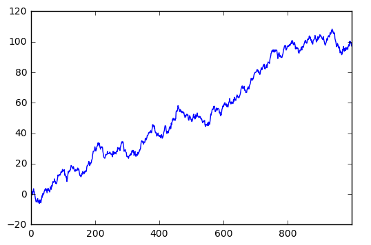
这是一个线性的数据,我们随机生成1000个数据,Series 默认的 index 就是从0开始的整数,但是这里我显式赋值以便让大家看的更清楚
# 随机生成1000个数据
data = pd.Series(np.random.randn(1000),index=np.arange(1000))

# 为了方便观看效果, 我们累加这个数据
data.cumsum()

# pandas 数据可以直接观看其可视化形式
data.plot()

plt.show()
就这么简单,熟悉 matplotlib 的朋友知道如果需要plot一个数据,我们可以使用 plt.plot(x=, y=),把x,y的数据作为参数存进去,但是data本来就是一个数据,所以我们可以直接plot。 生成的结果就是下图:
Dataframe 可视化
我们生成一个1000*4 的DataFrame,并对他们累加
data = pd.DataFrame(
    np.random.randn(1000,4),
    index=np.arange(1000),
    columns=list("ABCD")
    )
data.cumsum()
data.plot()
plt.show()
![[外链图片转存失败,源站可能有防盗链机制,建议将图片保存下来直接上传(img-5J67xUxC-1581681639878)(https://morvanzhou.github.io/static/results/np-pd/3-8-2.png)]](https://morvanzhou.github.io/static/results/np-pd/3-8-2.png)
这个就是我们刚刚生成的4个column的数据,因为有4组数据,所以4组数据会分别plot出来。plot 可以指定很多参数,具体的用法大家可以自己查一下这里
除了plot,我经常会用到还有scatter,这个会显示散点图,首先给大家说一下在 pandas 中有多少种方法
- bar
- hist
- box
- kde
- area
- scatter
- hexbin
但是我们今天不会一一介绍,主要说一下 plot 和 scatter. 因为scatter只有x,y两个属性,我们我们就可以分别给x, y指定数据
ax = data.plot.scatter(x='A',y='B',color='DarkBlue',label='Class1')
然后我们在可以再画一个在同一个ax上面,选择不一样的数据列,不同的 color 和 label
# 将之下这个 data 画在上一个 ax 上面
data.plot.scatter(x='A',y='C',color='LightGreen',label='Class2',ax=ax)
plt.show()
下面就是我plot出来的图片
![[外链图片转存失败,源站可能有防盗链机制,建议将图片保存下来直接上传(img-NWQRvMJB-1581681639879)(https://morvanzhou.github.io/static/results/np-pd/3-8-3.png)]](https://morvanzhou.github.io/static/results/np-pd/3-8-3.png)
这就是我们今天讲的两种呈现方式,一种是线性的方式,一种是散点图。