3.12 权重衰减

%matplotlib inline
import torch
import torch.nn as nn
import numpy as np
import sys
sys.path.append("..")
# import d2lzh_pytorch as d2l
print(torch.__version__)

3.12.2 高维线性回归试验

n_train, n_test, num_inputs = 20, 100, 200
true_w, true_b = torch.ones(num_inputs, 1)*0.01, 0.05

features = torch.randn((n_train + n_test, num_inputs))
labels = torch.matmul(features, true_w) + true_b
labels += torch.tensor(np.random.normal(0, 0.01, size=labels.size()), dtype=torch.float)
train_features, test_features = features[:n_train, :], features[n_train:, :]
train_labels, test_labels = labels[:n_train], labels[n_train:]

3.12.3 从零开始实现

3.12.3.1 初始化模型参数

def init_params():
    w = torch.randn((num_inputs, 1), requires_grad=True)
    b = torch.zeros(1, requires_grad=True)
    return [w, b]

3.12.3.2 定义L_2范数惩罚项

def l2_penalty(w):
    return (w**2).sum() / 2

3.12.3.3 定义训练和测试

def linreg(X, w, b):
    return torch.mm(X, w) + b

def squared_loss(y_hat, y): 
    # 注意这里返回的是向量, 另外, pytorch里的MSELoss并没有除以 2
    return ((y_hat - y.view(y_hat.size())) ** 2) / 2
def sgd(params, lr, batch_size):
    # 为了和原书保持一致，这里除以了batch_size，但是应该是不用除的，因为一般用PyTorch计算loss时就默认已经
    # 沿batch维求了平均了。
    for param in params:
        param.data -= lr * param.grad / batch_size # 注意这里更改param时用的param.data

from matplotlib import pyplot as plt
from IPython import display
def use_svg_display():
    """Use svg format to display plot in jupyter"""
    display.set_matplotlib_formats('svg')   # 设置图像显示格式为“svg”
    
def set_figsize(figsize=(3.5, 2.5)):
    use_svg_display()
    # 设置图的尺寸
    plt.rcParams['figure.figsize'] = figsize
def semilogy(x_vals, y_vals, x_label, y_label, x2_vals=None, y2_vals=None,
             legend=None, figsize=(3.5, 2.5)):
    set_figsize(figsize)
    plt.xlabel(x_label)
    plt.ylabel(y_label)
    plt.semilogy(x_vals, y_vals)
    if x2_vals and y2_vals:
        plt.semilogy(x2_vals, y2_vals, linestyle=':')
        plt.legend(legend)
    # plt.show()

batch_size, num_epochs, lr = 1, 100, 0.003
net, loss = linreg, squared_loss

dataset = torch.utils.data.TensorDataset(train_features, train_labels)
train_iter = torch.utils.data.DataLoader(dataset, batch_size, shuffle=True)

def fit_and_plot(lambd):
    w, b = init_params()
    train_ls , test_ls = [], []
    for _ in range(num_epochs):
        for X, y in train_iter:
            # 添加了L2范数惩罚项
            l = loss(net(X, w, b), y) + lambd * l2_penalty(w)
            l = l.sum()
            
            if w.grad is not None:
                w.grad.data.zero_()
                b.grad.data.zero_()
            l.backward()
            sgd([w, b], lr, batch_size)
        train_ls.append(loss(net(train_features, w, b), train_labels).mean().item())
        test_ls.append(loss(net(test_features, w, b), test_labels).mean().item())
    semilogy(range(1, num_epochs+1), train_ls, 'epochs', 'loss',
             range(1, num_epochs+1), test_ls, ['train', 'test'])
    print("L2 norm of w:", w.norm().item())

3.12.3.4 观察过拟合

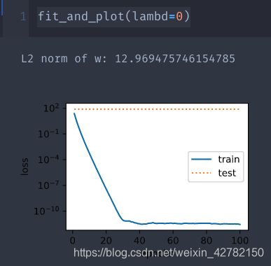
fit_and_plot(lambd=0)
>>>
L2 norm of w: 12.969475746154785

3.12.3.5 使用权重衰减

fit_and_plot(lambd=3)
>>>
L2 norm of w: 0.043992526829242706

3.12.4 简洁实现

def fit_and_plot_pytorch(wd):
    # 对权重衰减。权重名称一般是以weight结尾
    net = nn.Linear(num_inputs, 1)
    nn.init.normal_(net.weight, mean=0, std=1)
    nn.init.normal_(net.bias, mean=0, std=1)
    optimizer_w = torch.optim.SGD(params=[net.weight], lr=lr, weight_decay=wd) # 对权重参数衰减
    optimizer_b = torch.optim.SGD(params=[net.bias], lr=lr)   # 不对偏差参数衰减
    
    train_ls, test_ls = [], []
    for _ in range(num_epochs):
        for X, y in train_iter:
            l = loss(net(X), y).mean()
            optimizer_w.zero_grad()
            optimizer_b.zero_grad()
            
            l.backward()
            
            #对两个optimizer实例分别调用step函数，从而分别更新权重和偏差
            optimizer_w.step()
            optimizer_b.step()
        train_ls.append(loss(net(train_features), train_labels).mean().item())
        test_ls.append(loss(net(test_features),test_labels).mean().item())
    semilogy(range(1,num_epochs+1), train_ls, 'epochs', 'loss',
             range(1,num_epochs+1), test_ls, ['train', 'test'])
    print("L2 norm of w:", net.weight.data.norm().item())

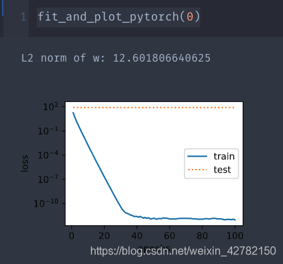
fit_and_plot_pytorch(0)
>>>
L2 norm of w: 12.601806640625

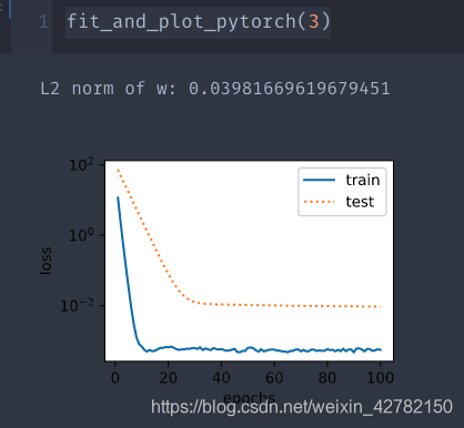
fit_and_plot_pytorch(3)
>>>
L2 norm of w: 0.03981669619679451