零 写在前面:
浏览器被不小心关闭了,编辑了半天的东西全没了,就简单写写吧,360真坑
object detection,就是在给定的图片中精确找到物体所在位置,并标注出物体的类别。再进一步简化说就是:
目标定位 + 识别
一,目标检测算法分类:
目前目标检测算法大体分为3类。
1.传统方法:
如adaboost+harr用来检测 hog + svm用来识别。
流程:a.穷举搜索框,设置目标大小范围以及高宽比例,穷举N种框。
b.提取特征如hog harr lbp等,将其归一化到固定尺寸如30*30这样 然后提取特征。
c.过分类器如adaboost ,svm等做最终分类。结果就是这个穷举的框的位置。
2.two stages:
代表作是R-CNN SPP-net Fast-RCNN Faster-RCNN R-FCN等等。演化过程是RCNN->SppNET->Fast-RCNN->Faster-RCNN,每个新版本都是为了解决老版本存在的一些致命问题而改进。
2.1. R-CNN算法介绍:
先说R-CNN算法,将深度学习引入了目标检测领域。
算法流程:
a.先弄个backbone,随便一个例如alexnet VGGnet等都行,确定下自己准备检测几类,就训练一个对应的分类网络或者直接fine-tuning一个现成网络改吧改吧。
b.利用选择性搜索方法select search提取待识别区域。这个select search算法是基于图分割的基础,利用各种规则做合并,得到的不同区域,疑似目标就包含在其中。减少了上面穷举法的弊端,搜索框限定在2000个左右,大大缩短时间了啊。对于每一个区域,修正区域大小以适合CNN的输入,做一次前向运算,将最后一个池化层的输出(就是对候选框提取到的特征)存到硬盘。
c.训练一个SVM分类器(二分类)来判断这个候选框里物体的类别每个类别对应一个SVM,判断是不是属于这个类别,是就是positive,反之nagative。
d.使用回归器精细修正候选框位置:对于每一个类,训练一个线性回归模型去判定这个框是否框得完美。边框回归详细介绍见我的博文:
显然R-CNN只是将神经网络作为一个特征提取器,最后识别是需要svm的,边框定位是用回归算法。
算法代码:没去特意关注,因为此算法显然不符合实际应用啊。
较上一版本改进点:鼻祖!
算法优缺点:深度学习进入目标检测领域。缺点很明显,2000个候选框看似少,但是每一个都输入CNN去做特征提取去,那效率比adaboost的穷举框不如啊。而且最后和adaboost一样是用svm做分类器的。
2.2. Fast R-CNN算法介绍:
Fast R-CNN 要先说下sppnet。sppnet是为了解决任意尺寸输入而生,输入数据每次都需要放缩到固定大小以适应全连接层,而放缩会导致目标形变,形变肯定影响识别结果啊。详细SPPnet看我的博文https://blog.csdn.net/gbz3300255/article/details/105843416
算法流程:
a.与RCNN一样
b.前半部分select search提取待识别区域与RCNN一致,后面将整图都输入CNN网络中去提取特征了。这样就不用做2000多次特征提取了,一次就完事了,然后按框与特征图的映射关系去提取每一部分的特征图就好
c.2000多个小patch对应的特征图直接分别放入sppnet,获得输出特征就好,不用对提取出的小patch进行resize了。
d.后面一样了,过svm分类器去做类别判断,用边框回归方法做位置修正。
算法代码:没去特意关注,因为此算法显然不符合实际应用啊。
较上一版本改进点:显然fast R-CNN 特征提取部分做了大修正,特征提取一次且不用对其resize,提升了效率和准确性
算法优缺点:较上一版本效率提升,准确率提升,还是略显麻烦,不易用啊。
2.3. Faster R-CNN算法介绍:
Fast R-CNN 看上去很美,但前面那个选择性搜索耗时还是多,想法让这个搜索也网络来做就好了,就有大神提出了RPN网络,RPN网络说白了就是一个粗搜索的网络框架,输出结果是一堆候选框,详情可看我的博文:https://mp.csdn.net/console/editor/html/105493407
算法流程:
a. 对整张图片输进CNN,得到feature map
b. 将卷积特征feature map输入到RPN,得到候选框的特征信息。
c. 对候选框中提取出的特征,使用分类器判别是否属于一个特定类
d. 对于属于某一特征的候选框,用回归器进一步调整其位置
算法代码:没去特意关注,因为此算法显然不符合实际应用啊。
较上一版本改进点:显然去掉了候选框在外面提取的步骤,将此步骤用神经网络完成,进一步简化了步骤,算法性能又进一步提升了
算法优缺点:较上一版本效率提升,准确率提升,初步可用。
3.one stages:
3.1 yolov1
上面的两阶段法效率低下,有大神提出了YOLO检测算法,该方法基于回归,一次将检测和识别搞定,所以叫one stages方法。you only look once。one stages 的开山之作。
算法流程:
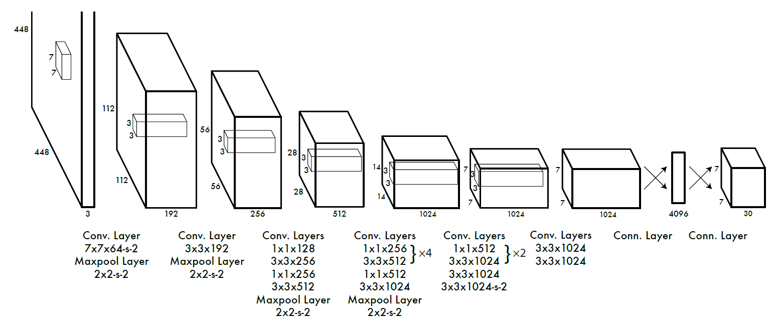
a. 如下图,输入图像大小为448*448,经过若干个卷积层与池化层,变为7*7*1024张量(图一中倒数第三个立方体),最后经过两层全连接层,输出张量维度为7*7*N,这就是Yolo v1的整个神经网络结构。这个N与检测类别有关,计算公式为:7 * 7 * (框个数 * 5 + 类别数那么多的置信度) 其中5为框的坐标 (x0,y0)(x1,y1) + 框存在的置信度。具体例子:例如要检测10类,每个锚点有2种框(长宽比为1:2与2:1).那么就是7*7*(2 * 5 + 10)。yolov1的锚点框大小是人为设定的哦,v2v3开始是用聚类方法自己算的,更符合实际应用感觉。
b.进行非极大值抑制,筛选Boxes,作为输出结果。非极大值抑说白了就是去除重叠的伪结果。非极大值抑制流程:(1)将所有框的得分排序,选中最高分及其对应的框 (2)遍历其余的框,如果和当前最高分框的重叠面积(IOU)大于一定阈值,我们就将框删除。 (3)从未处理的框中继续选一个得分最高的,重复上述过程。
算法代码:没去特意关注,因为直接看的yolov3哈哈。v1是开山之作但小目标检测效果差。
算法损失函数:
损失函数的设计目标就是让坐标(x,y,w,h),confidence,classification 这个三个方面达到很好的平衡。 简单的全部采用了sum-squared error loss来做这件事会有以下不足: a) 8维的localization error和20维的classification error同等重要显然是不合理的。 b) 如果一些栅格中没有object(一幅图中这种栅格很多),那么就会将这些栅格中的bounding box的confidence 置为0,相比于较少的有object的栅格,这些不包含物体的栅格对梯度更新的贡献会远大于包含物体的栅格对梯度更新的贡献,这会导致网络不稳定甚至发散。

更重视8维的坐标预测,给这些损失前面赋予更大的loss weight, 记为 λcoord ,在pascal VOC训练中取5。(上图蓝色框)
对没有object的bbox的confidence loss,赋予小的loss weight,记为 λnoobj ,在pascal VOC训练中取0.5。(上图橙色框)
有object的bbox的confidence loss (上图红色框) 和类别的loss (上图紫色框)的loss weight正常取1。
找了个yolov1的损失函数pytorch版本的,加深下理解吧。
首先明确一概念,网格就是最终特征图(7*7*30)上的一个预测目标了,v1版本这样的预测结果网格一共有49个,每个维度为1*30.这30的向量含义为【x0,y0,w0, h0,I0,x1,y1,w1, h1,I1,C0,C1,C2.....C19】前面10位代表了2个box框信息以及其置信度,后20位表示了分类概率值。后面的损失函数都是针对网格中的一些属性来干活的。
a.标注图像某位置有目标,预测为有==>计算not response loss 未响应损失以及box框的坐标等的信息对应红色框和蓝色框
coo_response_mask = torch.cuda.ByteTensor(box_target.size())
coo_response_mask.zero_()
coo_not_response_mask = torch.cuda.ByteTensor(box_target.size())
coo_not_response_mask.zero_()
for i in range(0,box_target.size()[0],2):
	box1 = box_pred[i:i+2]
	box1_xyxy = Variable(torch.FloatTensor(box1.size()))
	box1_xyxy[:,:2] = box1[:,:2] -0.5*box1[:,2:4]
	box1_xyxy[:,2:4] = box1[:,:2] +0.5*box1[:,2:4]
	box2 = box_target[i].view(-1,5)
	box2_xyxy = Variable(torch.FloatTensor(box2.size()))
	box2_xyxy[:,:2] = box2[:,:2] -0.5*box2[:,2:4]
	box2_xyxy[:,2:4] = box2[:,:2] +0.5*box2[:,2:4]
	iou = self.compute_iou(box1_xyxy[:,:4],box2_xyxy[:,:4]) #[2,1]
	max_iou,max_index = iou.max(0)
	max_index = max_index.data.cuda()
	coo_response_mask[i+max_index]=1
	coo_not_response_mask[i+1-max_index]=1
box_pred_response = box_pred[coo_response_mask].view(-1,5)
box_target_response = box_target[coo_response_mask].view(-1,5)
contain_loss = F.mse_loss(box_pred_response[:,4],box_target_response[:,4],size_average=False)
loc_loss = F.mse_loss(box_pred_response[:,:2],box_target_response[:,:2],size_average=False) + F.mse_loss(torch.sqrt(box_pred_response[:,2:4]),torch.sqrt(box_target_response[:,2:4]),size_average=False)contain_loss是计算预测为有目标的网格的confidence与真值的confidence的平方误差作为loss判定。只是两个值的计算对应红色框。
loc_loss是计算蓝色框的内容呢。
b.标注图像某位置有目标,预测为无==>计算response loss响应损失,对应代码。
box_pred_not_response = box_pred[coo_not_response_mask].view(-1,5)
box_target_not_response = box_target[coo_not_response_mask].view(-1,5)
not_contain_loss = F.mse_loss(box_pred_response[:,4],box_target_response[:,4],size_average=False)not_contain_loss是计算预测为无的网格confidence与真值的confidence的平方误差作为loss判定,也只是两个值的计算对应红色框。 可见红色框是分了两部分计算的切记切记
c.标注图像某位置无目标,预测为有==>计算不包含obj损失 只计算第4,9位的有无物体概率的loss ,对应代码是下面这行。
noo_pred = pred_tensor[noo_mask].view(-1,30)
noo_target = target_tensor[noo_mask].view(-1,30)
noo_pred_mask = torch.cuda.ByteTensor(noo_pred.size())
noo_pred_mask.zero_()
# 将第4、9  即有物体的confidence置为1
noo_pred_mask[:, 4] = 1
noo_pred_mask[:, 9] = 1
noo_pred_c = noo_pred[noo_pred_mask]
noo_target_c = noo_target[noo_pred_mask]
nooobj_loss = F.mse_loss(noo_pred_c,noo_target_c,size_average=False)
noo_mask记录的是所有网格在真实图像上目标存在与否的标签。
noo_pred是根据noo_mask标签取出的实际不含目标的预测网格的向量。其向量4,,9位置的值是预测值。
noo_target是根据noo_mask标签取出的实际不含目标的真值网格的向量。其向量第4 ,9位置值是0。
nooobj_loss只计算了这个些网格30维向量的4,9位置的损失值,其他位置都没用。对应上图中的橙色框。这样此部分的loss函数目标就是让预测值越接近0越好。符合了loss的目的了
d.标注图像某位置无目标,预测为无==>无损失(不计算)
e 类别的损失函数计算,代码如下:
class_loss = F.mse_loss(class_pred, class_target, size_average=False)class_loss计算的是类别的损失函数,是网格向量的后20个数据做最小平方误差来构建loss函数的。对应图中紫色框
至此v1的损失函数整体就完事了呀。
目标检测神经网络的损失函数就用上面这4部分组成了。后续网络优化目的就是计量减少这个函数的值,换句话说就是如果此区域存在真值,就训练出一组权重让预测中心无限接近真值中心,让预测边框无限接近真值边框。
较上一版本改进点:真正的端到端的训练,开山之作,准确率不足,效率飞升。
算法优缺点:较上一版本效率提升,工业应用可期。但是它只在7*7这个特征图上做文章,丢失很多细节,也是小目标检测能力低下的根本原因。定位精度低,每个框内只能检出一个目标(例如鸟群)。略显粗糙啊。还有其用了全连接层,所以输入数据需要放缩到统一尺度才能进行检测。
3.2 SSD
应该介绍v2,结果ssd横插一扛子,因为它对标的就是v1,解决了v1定位不准问题。然后yolov2又吊打它.........。
SSD从YOLOV1中继承了将detection转化为regression的思路,一次完成目标定位与分类。基于Faster RCNN中的Anchor,提出了相似的Prior box;加入基于特征金字塔(Pyramidal Feature Hierarchy)的检测方式,即在不同感受野的feature map上预测目标,增加了小目标检测能力,但是因为小目标检测用的是低层特征,非线性表达能力欠缺,还不能达到很高的精度。
算法流程:
a. 将整张图片输入VGG网络前半部分,得到A部分输出,其输出是relu之后的结果, 尺寸为38 * 38 * 512,在其上做一次Normalization,然后对此特征图做分类预测和边框的回归计算,输出A1。
b.将A部分作为输入放入VGG网络后半部分,其输出也是relu之后的结果记为B, 尺寸为19* 19 * 1024,然后对此特征图做分类预测和边框的回归计算,输出B1。
c. 将B部分作为输入放入extras网络,其输出都是卷积结果 记录C D E F, 尺寸分别为10*10*512 5 *5 * 256 3*3 *256 1*1*256,然后对此特征图做分类预测和边框的回归计算,输出分别为C1 D1 E1 F1。
d. 用非极大值抑制对结果做一次抑制,输出最终结果就是检测结果了
e. 上面是写的SSD的主要流程,这里漏写了一个detector classfiler具体怎么实现,其中涉及了anchor的设置等等,这块是SSD的一个重点。下面这个是anchor的计算方法

SSD的配置文件如下。上图的ratio对应anchor_ratios。 min_size 与max_size对应anchor_sizes。anchor_ratios决定着长方形框个数(分别是2,4,4,4,2,2),anchor_sizes决定正方形框个数(固定2个)
default_params = SSDParams(
        img_shape=(300, 300),
        num_classes=21,
        no_annotation_label=21,
        feat_layers=['block4', 'block7', 'block8', 'block9', 'block10', 'block11'],
        feat_shapes=[(38, 38), (19, 19), (10, 10), (5, 5), (3, 3), (1, 1)],
        anchor_size_bounds=[0.15, 0.90],
        # anchor_size_bounds=[0.20, 0.90],
        anchor_sizes=[(21., 45.),
                      (45., 99.),
                      (99., 153.),
                      (153., 207.),
                      (207., 261.),
                      (261., 315.)],
        # anchor_sizes=[(30., 60.),
        #               (60., 111.),
        #               (111., 162.),
        #               (162., 213.),
        #               (213., 264.),
        #               (264., 315.)],
        anchor_ratios=[[2, .5],
                       [2, .5, 3, 1./3],
                       [2, .5, 3, 1./3],
                       [2, .5, 3, 1./3],
                       [2, .5],
                       [2, .5]],
        anchor_steps=[8, 16, 32, 64, 100, 300],
        anchor_offset=0.5,
        normalizations=[20, -1, -1, -1, -1, -1],
        prior_scaling=[0.1, 0.1, 0.2, 0.2]
        )
f.损失函数:

具体解释:公式1组成部分为 框位置损失(公式2) + 存在损失(公式3),具体内容如上图。所谓损失函数就是想让这个函数值越小越好。
算法的详细流程如下图所示:

算法代码:
A部分下面这行的输出
(vgg): ModuleList
(22): ReLU(inplace=True)B部分下面这行的输出
(vgg): ModuleList
(34): ReLU(inplace=True)
C D E F部分是下面这几行对应的
(extras): ModuleList的
(1): Conv2d(256, 512, kernel_size=(3, 3), stride=(2, 2), padding=(1, 1))
(3): Conv2d(128, 256, kernel_size=(3, 3), stride=(2, 2), padding=(1, 1))
(5): Conv2d(128, 256, kernel_size=(3, 3), stride=(1, 1))
(7): Conv2d(128, 256, kernel_size=(3, 3), stride=(1, 1))
SSD的网络结构如下:
SSD(
  (vgg): ModuleList(
    (0): Conv2d(3, 64, kernel_size=(3, 3), stride=(1, 1), padding=(1, 1))
    (1): ReLU(inplace=True)
    (2): Conv2d(64, 64, kernel_size=(3, 3), stride=(1, 1), padding=(1, 1))
    (3): ReLU(inplace=True)
    (4): MaxPool2d(kernel_size=2, stride=2, padding=0, dilation=1, ceil_mode=False)
    (5): Conv2d(64, 128, kernel_size=(3, 3), stride=(1, 1), padding=(1, 1))
    (6): ReLU(inplace=True)
    (7): Conv2d(128, 128, kernel_size=(3, 3), stride=(1, 1), padding=(1, 1))
    (8): ReLU(inplace=True)
    (9): MaxPool2d(kernel_size=2, stride=2, padding=0, dilation=1, ceil_mode=False)
    (10): Conv2d(128, 256, kernel_size=(3, 3), stride=(1, 1), padding=(1, 1))
    (11): ReLU(inplace=True)
    (12): Conv2d(256, 256, kernel_size=(3, 3), stride=(1, 1), padding=(1, 1))
    (13): ReLU(inplace=True)
    (14): Conv2d(256, 256, kernel_size=(3, 3), stride=(1, 1), padding=(1, 1))
    (15): ReLU(inplace=True)
    (16): MaxPool2d(kernel_size=2, stride=2, padding=0, dilation=1, ceil_mode=True)
    (17): Conv2d(256, 512, kernel_size=(3, 3), stride=(1, 1), padding=(1, 1))
    (18): ReLU(inplace=True)
    (19): Conv2d(512, 512, kernel_size=(3, 3), stride=(1, 1), padding=(1, 1))
    (20): ReLU(inplace=True)
    (21): Conv2d(512, 512, kernel_size=(3, 3), stride=(1, 1), padding=(1, 1))
    (22): ReLU(inplace=True)
    (23): MaxPool2d(kernel_size=2, stride=2, padding=0, dilation=1, ceil_mode=False)
    (24): Conv2d(512, 512, kernel_size=(3, 3), stride=(1, 1), padding=(1, 1))
    (25): ReLU(inplace=True)
    (26): Conv2d(512, 512, kernel_size=(3, 3), stride=(1, 1), padding=(1, 1))
    (27): ReLU(inplace=True)
    (28): Conv2d(512, 512, kernel_size=(3, 3), stride=(1, 1), padding=(1, 1))
    (29): ReLU(inplace=True)
    (30): MaxPool2d(kernel_size=3, stride=1, padding=1, dilation=1, ceil_mode=False)
    (31): Conv2d(512, 1024, kernel_size=(3, 3), stride=(1, 1), padding=(6, 6), dilation=(6, 6))
    (32): ReLU(inplace=True)
    (33): Conv2d(1024, 1024, kernel_size=(1, 1), stride=(1, 1))
    (34): ReLU(inplace=True)
  )
  (L2Norm): L2Norm()
  (extras): ModuleList(
    (0): Conv2d(1024, 256, kernel_size=(1, 1), stride=(1, 1))
    (1): Conv2d(256, 512, kernel_size=(3, 3), stride=(2, 2), padding=(1, 1))
    (2): Conv2d(512, 128, kernel_size=(1, 1), stride=(1, 1))
    (3): Conv2d(128, 256, kernel_size=(3, 3), stride=(2, 2), padding=(1, 1))
    (4): Conv2d(256, 128, kernel_size=(1, 1), stride=(1, 1))
    (5): Conv2d(128, 256, kernel_size=(3, 3), stride=(1, 1))
    (6): Conv2d(256, 128, kernel_size=(1, 1), stride=(1, 1))
    (7): Conv2d(128, 256, kernel_size=(3, 3), stride=(1, 1))
  )
  (loc): ModuleList(
    (0): Conv2d(512, 16, kernel_size=(3, 3), stride=(1, 1), padding=(1, 1))
    (1): Conv2d(1024, 24, kernel_size=(3, 3), stride=(1, 1), padding=(1, 1))
    (2): Conv2d(512, 24, kernel_size=(3, 3), stride=(1, 1), padding=(1, 1))
    (3): Conv2d(256, 24, kernel_size=(3, 3), stride=(1, 1), padding=(1, 1))
    (4): Conv2d(256, 16, kernel_size=(3, 3), stride=(1, 1), padding=(1, 1))
    (5): Conv2d(256, 16, kernel_size=(3, 3), stride=(1, 1), padding=(1, 1))
  )
  (conf): ModuleList(
    (0): Conv2d(512, 84, kernel_size=(3, 3), stride=(1, 1), padding=(1, 1))
    (1): Conv2d(1024, 126, kernel_size=(3, 3), stride=(1, 1), padding=(1, 1))
    (2): Conv2d(512, 126, kernel_size=(3, 3), stride=(1, 1), padding=(1, 1))
    (3): Conv2d(256, 126, kernel_size=(3, 3), stride=(1, 1), padding=(1, 1))
    (4): Conv2d(256, 84, kernel_size=(3, 3), stride=(1, 1), padding=(1, 1))
    (5): Conv2d(256, 84, kernel_size=(3, 3), stride=(1, 1), padding=(1, 1))
  )
)
主要代码如下,为了看算法方便,摘了下代码,主要是为了看上面那个图的 图像数据流处理流程。最后那个文件是可以直接运行的。
这部分代码是VGG网络的。通过打印可以看到VGG网络的各行执行哪些操作。
def vgg(cfg, i, batch_norm=False):
    layers = []
    in_channels = i
    for v in cfg:
        if v == 'M':
            layers += [nn.MaxPool2d(kernel_size=2, stride=2)]
        elif v == 'C':
            layers += [nn.MaxPool2d(kernel_size=2, stride=2, ceil_mode=True)]
        else:
            conv2d = nn.Conv2d(in_channels, v, kernel_size=3, padding=1)
            if batch_norm:
                layers += [conv2d, nn.BatchNorm2d(v), nn.ReLU(inplace=True)]
            else:
                layers += [conv2d, nn.ReLU(inplace=True)]
            in_channels = v
    pool5 = nn.MaxPool2d(kernel_size=3, stride=1, padding=1)
    conv6 = nn.Conv2d(512, 1024, kernel_size=3, padding=6, dilation=6)
    conv7 = nn.Conv2d(1024, 1024, kernel_size=1)
    layers += [pool5, conv6,
               nn.ReLU(inplace=True), conv7, nn.ReLU(inplace=True)]
    return layers
这部分代码是extras网络的。通过打印可以看到extras网络的各行执行哪些操作。是在VGG网络后又加了个尾巴。
def add_extras(cfg, i, batch_norm=False):
    # Extra layers added to VGG for feature scaling
    layers = []
    in_channels = i
    flag = False
    for k, v in enumerate(cfg):
        if in_channels != 'S':
            if v == 'S':
                layers += [nn.Conv2d(in_channels, cfg[k + 1],
                           kernel_size=(1, 3)[flag], stride=2, padding=1)]
            else:
                layers += [nn.Conv2d(in_channels, v, kernel_size=(1, 3)[flag])]
            flag = not flag
        in_channels = v
    return layers
生成VGG+extras网络 代码如下。通过这个将上面两个网络生成出来。
def multibox(vgg, extra_layers, cfg, num_classes):
    loc_layers = []
    conf_layers = []
    vgg_source = [21, -2]
    for k, v in enumerate(vgg_source):
        loc_layers += [nn.Conv2d(vgg[v].out_channels,
                                 cfg[k] * 4, kernel_size=3, padding=1)]

        conf_layers += [nn.Conv2d(vgg[v].out_channels,
                        cfg[k] * num_classes, kernel_size=3, padding=1)]

    for k, v in enumerate(extra_layers[1::2], 2):
        loc_layers += [nn.Conv2d(v.out_channels, cfg[k]
                                 * 4, kernel_size=3, padding=1)]
        conf_layers += [nn.Conv2d(v.out_channels, cfg[k]
                                  * num_classes, kernel_size=3, padding=1)]
    print("loc_layers =", loc_layers)
    return vgg, extra_layers, (loc_layers, conf_layers)
总的可运行代码如下:
#encoding=utf-8
import torch
import torch.nn as nn
import torch.nn.functional as F
from torch.autograd import Variable
#from data import voc, coco
import os

from torch.autograd import Function
import torch.nn.init as init

class L2Norm(nn.Module):
    def __init__(self,n_channels, scale):
        super(L2Norm,self).__init__()
        self.n_channels = n_channels
        self.gamma = scale or None
        self.eps = 1e-10
        self.weight = nn.Parameter(torch.Tensor(self.n_channels))
        self.reset_parameters()

    def reset_parameters(self):
        init.constant_(self.weight,self.gamma)

    def forward(self, x):
        norm = x.pow(2).sum(dim=1, keepdim=True).sqrt()+self.eps
        #x /= norm
        x = torch.div(x,norm)
        out = self.weight.unsqueeze(0).unsqueeze(2).unsqueeze(3).expand_as(x) * x
        return out

class SSD(nn.Module):
    """Single Shot Multibox Architecture
    The network is composed of a base VGG network followed by the
    added multibox conv layers.  Each multibox layer branches into
        1) conv2d for class conf scores
        2) conv2d for localization predictions
        3) associated priorbox layer to produce default bounding
           boxes specific to the layer's feature map size.
    See: https://arxiv.org/pdf/1512.02325.pdf for more details.

    Args:
        phase: (string) Can be "test" or "train"
        size: input image size
        base: VGG16 layers for input, size of either 300 or 500
        extras: extra layers that feed to multibox loc and conf layers
        head: "multibox head" consists of loc and conf conv layers
    """

    def __init__(self, phase, size, base, extras, head, num_classes):
        super(SSD, self).__init__()
        self.phase = phase
        self.num_classes = num_classes
        #self.cfg = (coco, voc)[num_classes == 21]
        #self.priorbox = PriorBox(self.cfg)
        #self.priors = Variable(self.priorbox.forward(), volatile=True)
        self.size = size

        # SSD network
        self.vgg = nn.ModuleList(base)
        # Layer learns to scale the l2 normalized features from conv4_3
        self.L2Norm = L2Norm(512, 20)
        self.extras = nn.ModuleList(extras)

        self.loc = nn.ModuleList(head[0])
        self.conf = nn.ModuleList(head[1])

        #if phase == 'test':
            #self.softmax = nn.Softmax(dim=-1)
            #self.detect = Detect(num_classes, 0, 200, 0.01, 0.45)

    def forward(self, x):
        """Applies network layers and ops on input image(s) x.

        Args:
            x: input image or batch of images. Shape: [batch,3,300,300].

        Return:
            Depending on phase:
            test:
                Variable(tensor) of output class label predictions,
                confidence score, and corresponding location predictions for
                each object detected. Shape: [batch,topk,7]

            train:
                list of concat outputs from:
                    1: confidence layers, Shape: [batch*num_priors,num_classes]
                    2: localization layers, Shape: [batch,num_priors*4]
                    3: priorbox layers, Shape: [2,num_priors*4]
        """
        sources = list()
        loc = list()
        conf = list()

        # apply vgg up to conv4_3 relu
        for k in range(23):
            x = self.vgg[k](x)
        s = self.L2Norm(x)
        sources.append(s)#对应图中的38*38*512那个分支的检测 最终的结果是在relu处理之后maxpool处理之前
        # apply vgg up to fc7
        for k in range(23, len(self.vgg)):
            x = self.vgg[k](x)
        #print("x1 = ", x.shape)
        sources.append(x)#对应图中的19*19*1024那个分支的检测


        # apply extra layers and cache source layer outputs
        for k, v in enumerate(self.extras):
            x = F.relu(v(x), inplace=True)
            if k % 2 == 1:
                sources.append(x)#对应图中的10*10*512  5*5*256  3*3*256 1*1*256 那4个分支的检测
                #print("k = ", self.extras[k])

        # apply multibox head to source layers
        for (x, l, c) in zip(sources, self.loc, self.conf):
            loc.append(l(x).permute(0, 2, 3, 1).contiguous())
            conf.append(c(x).permute(0, 2, 3, 1).contiguous())

        loc = torch.cat([o.view(o.size(0), -1) for o in loc], 1)
        conf = torch.cat([o.view(o.size(0), -1) for o in conf], 1)

        '''
        if self.phase == "test":
            output = self.detect(
                loc.view(loc.size(0), -1, 4),                   # loc preds
                self.softmax(conf.view(conf.size(0), -1,
                             self.num_classes)),                # conf preds
                self.priors.type(type(x.data))                  # default boxes
            )
        else:
            output = (
                loc.view(loc.size(0), -1, 4),
                conf.view(conf.size(0), -1, self.num_classes),
                self.priors
            )
        '''
        return conf

    def load_weights(self, base_file):
        other, ext = os.path.splitext(base_file)
        if ext == '.pkl' or '.pth':
            print('Loading weights into state dict...')
            self.load_state_dict(torch.load(base_file,
                                 map_location=lambda storage, loc: storage))
            print('Finished!')
        else:
            print('Sorry only .pth and .pkl files supported.')


def vgg(cfg, i, batch_norm=False):
    layers = []
    in_channels = i
    for v in cfg:
        if v == 'M':
            layers += [nn.MaxPool2d(kernel_size=2, stride=2)]
        elif v == 'C':
            layers += [nn.MaxPool2d(kernel_size=2, stride=2, ceil_mode=True)]
        else:
            conv2d = nn.Conv2d(in_channels, v, kernel_size=3, padding=1)
            if batch_norm:
                layers += [conv2d, nn.BatchNorm2d(v), nn.ReLU(inplace=True)]
            else:
                layers += [conv2d, nn.ReLU(inplace=True)]
            in_channels = v
    pool5 = nn.MaxPool2d(kernel_size=3, stride=1, padding=1)
    conv6 = nn.Conv2d(512, 1024, kernel_size=3, padding=6, dilation=6)
    conv7 = nn.Conv2d(1024, 1024, kernel_size=1)
    layers += [pool5, conv6,
               nn.ReLU(inplace=True), conv7, nn.ReLU(inplace=True)]
    return layers


def add_extras(cfg, i, batch_norm=False):
    # Extra layers added to VGG for feature scaling
    layers = []
    in_channels = i
    flag = False
    for k, v in enumerate(cfg):
        if in_channels != 'S':
            if v == 'S':
                layers += [nn.Conv2d(in_channels, cfg[k + 1],
                           kernel_size=(1, 3)[flag], stride=2, padding=1)]
            else:
                layers += [nn.Conv2d(in_channels, v, kernel_size=(1, 3)[flag])]
            flag = not flag
        in_channels = v
    return layers


def multibox(vgg, extra_layers, cfg, num_classes):
    loc_layers = []
    conf_layers = []
    vgg_source = [21, -2]
    for k, v in enumerate(vgg_source):
        loc_layers += [nn.Conv2d(vgg[v].out_channels,
                                 cfg[k] * 4, kernel_size=3, padding=1)]

        conf_layers += [nn.Conv2d(vgg[v].out_channels,
                        cfg[k] * num_classes, kernel_size=3, padding=1)]

    for k, v in enumerate(extra_layers[1::2], 2):
        loc_layers += [nn.Conv2d(v.out_channels, cfg[k]
                                 * 4, kernel_size=3, padding=1)]
        conf_layers += [nn.Conv2d(v.out_channels, cfg[k]
                                  * num_classes, kernel_size=3, padding=1)]
    print("loc_layers =", loc_layers)
    return vgg, extra_layers, (loc_layers, conf_layers)


base = {
    '300': [64, 64, 'M', 128, 128, 'M', 256, 256, 256, 'C', 512, 512, 512, 'M',
            512, 512, 512],
    '512': [],
}
extras = {
    '300': [256, 'S', 512, 128, 'S', 256, 128, 256, 128, 256],
    '512': [],
}

mbox = {
    '300': [4, 6, 6, 6, 4, 4],  # number of boxes per feature map location  每个输出层的框个数
    '512': [],
}

def process():
	size=300
	num_classes=21
	phase = "train"
	base_, extras_, head_ = multibox(vgg(base[str(size)], 3),add_extras(extras[str(size)], 1024),mbox[str(size)], num_classes)


	XXX = SSD(phase, size, base_, extras_, head_, num_classes)
	print(XXX)
	return XXX

if __name__ == '__main__':
	ssd_net = process()
	#ssd_net = build_ssd('train', cfg['min_dim'], cfg['num_classes'])
	images = torch.randn(1,3,300,300)
	out = ssd_net(images)
	print("process end")
具体怎么训练,怎么测试就没去关注了因为后面的yolov2开始就吊打它了。没去详细看了
损失函数:
算法优缺点:准确率高于yolov1,低于yolov2
3.3 YOLOV2
YOLOv2主要改进是提高召回率和定位能力,V2相比V1提高了输入的分辨率,采用了自己定义的darknet网络作为backbone,V2借鉴Faster R-CNN的思想预测bbox的偏移.移除了全连接层,并且删掉了一个pooling层使特征的分辨率更大一些,V2对Faster R-CNN的手选先验框方法做了改进,采用聚类的方法确定先验框,使用聚类进行选择的优势是达到相同的IOU结果时所需的anchor box数量更少,使得模型的表示能力更强,任务更容易学习。在Faster R-CNN 和 SSD 均使用了不同的feature map以适应不同尺度大小的目标.YOLOv2使用了一种不同的方法,简单添加一个 pass through layer,把浅层特征图(26x26)连接到深层特征图(连接到新加入的三个卷积核尺寸为3 * 3的卷积层最后一层的输入)。 通过叠加浅层特征图相邻特征到不同通道(而非空间位置),类似于Resnet中的identity mapping。这个方法把26x26x512的特征图叠加成13x13x2048的特征图,与原生的深层特征图相连接,使模型有了细粒度特征。此方法使得模型的性能获得了提升。和YOLOv1训练时网络输入的图像尺寸固定不变不同,YOLOv2(在cfg文件中random=1时)每隔几次迭代后就会微调网络的输入尺寸。训练时每迭代10次,就会随机选择新的输入图像尺寸。因为YOLOv2的网络使用的downsamples倍率为32,所以使用32的倍数调整输入图像尺寸{320,352,…,608}。训练使用的最小的图像尺寸为320 x 320,最大的图像尺寸为608 x 608。 这使得网络可以适应多种不同尺度的输入.
yolo v1中是没有使用到anchor的,这使得每个网格中的每个cell只能预测一个物体。因此yolo v2借鉴了faster RCNN中anchor的思想,这样实际上使得grid的每个cell可以预测多个尺度的不同物体。yolo v1中grid的大小是7x7,但是yolo v2的grid变成了13x13,grid中的每个cell都对应这5个不同尺寸的anchor。
算法流程:

网络抛弃了全连接,采用全卷积FCN的架构,因此可以输入任意大小的图片。在每个卷积层之后都使用了BN。BN的作用是为了是网络更容易收敛,除此之外还有正则化的作用,可以防止过拟合。
使用了跨层连接,这个借鉴了ResNet的identity mapping思想。跨层连接的一个大好处是使梯度更容易前传,也就是说可以让网络训练变得更容易。但是,这个跨层连接有点别致,一般的跨层连接,会通过求和或者通道连接进行特征融合,但是yolov2在融合之前还添加了一个reorganization的操作。经过这样的操作,实际上已经把feature map的排布重整了,直觉上觉得这么做不太好,但事实证明它是可行的。不过这么做的一个好处就是将所有的信息都传递到后面的层,并没有因为下采样等操作导致损失信息,因此获得了更多细粒度的特征。
那什么是reorganization层?其实很简单,就是将大分辨率的feature map进行重新排布得到分辨率更小的feature map,相应的通道数增加。举例来说,如果网络的输入维度是3x416x416,那么conv13_512的维度则是512x26x26,将其进行重新排布之后则变成2048x13x13。这个重新排布如图:
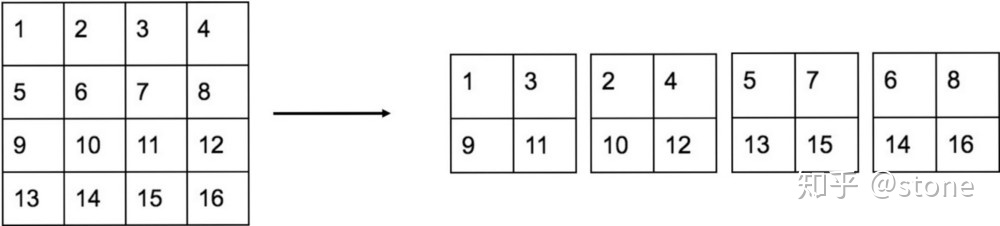
实际上就是将一个feature map变成了更小的feature map,但是通道数变多了。
假设网络图片的输入大小是[416,416],那么经过骨架网络(或者说特征提取网络)之后,由于存在步长为32的分辨率降低,这样网络的输出是[13,13,1024]。要将其转化为预测,使用一个1x1的卷积将通道数压缩到
1024-->(num_anchor x * (4+1+num_class),如下图所示)这个维度就可以了,这里的num_anchor表示feature map上每个点对应的anchor数目,4表示x y w h 属于box信息,1表示confidence,num_class表示预测的类别数,注意这里的类别数是不包括背景。

实际上,这个还不是真正预测的输出结果,这个输出结果需要进行一定的转换,在介绍转换之前,需要讲解anchor,因为转换是基于anchor来进行的。
算法代码:https://github.com/longcw/yolo2-pytorch
损失函数:没去看论文,直接看上面代码了,1.4k的点赞量的代码,损失函数包含三部分 框的损失 iou损失(存在损失) 类别损失三类。代码如下:调用关系是_build_target是入口。其调用_process_batch函数。_process_batch函数具体实现了这三类损失计算前的准备工作。如预测框的选择,预测框iou的计算(找与真值最匹配的anchor框),乘以权重等都在这里面算的。具体写了一部分注释,没耐心细看下去了。
import torch
import numpy as np
import torch.nn as nn
import torch.nn.functional as F

import utils.network as net_utils
import cfgs.config as cfg
from layers.reorg.reorg_layer import ReorgLayer
from utils.cython_bbox import bbox_ious, anchor_intersections
from utils.cython_yolo import yolo_to_bbox
from functools import partial

from multiprocessing import Pool


def _make_layers(in_channels, net_cfg):
    layers = []

    if len(net_cfg) > 0 and isinstance(net_cfg[0], list):
        for sub_cfg in net_cfg:
            layer, in_channels = _make_layers(in_channels, sub_cfg)
            layers.append(layer)
    else:
        for item in net_cfg:
            if item == 'M':
                layers.append(nn.MaxPool2d(kernel_size=2, stride=2))
            else:
                out_channels, ksize = item
                layers.append(net_utils.Conv2d_BatchNorm(in_channels,
                                                         out_channels,
                                                         ksize,
                                                         same_padding=True))
                # layers.append(net_utils.Conv2d(in_channels, out_channels,
                #     ksize, same_padding=True))
                in_channels = out_channels

    return nn.Sequential(*layers), in_channels


def _process_batch(data, size_index):
    W, H = cfg.multi_scale_out_size[size_index]#特征图尺寸呗 决定于size_index参数
    inp_size = cfg.multi_scale_inp_size[size_index] #输入图像尺寸
    out_size = cfg.multi_scale_out_size[size_index] #输出图像 也就是特征图的尺寸
    #bbox_pred_np:边框预测值   gt_boxes:  空 边框真值    gt_classes: 类别真值    dontcares:  空  iou_pred_np:  IOU预测值
    bbox_pred_np, gt_boxes, gt_classes, dontcares, iou_pred_np = data #获得网格的特征图数据 包括

    # net output
    #bbox_pred_np 的shape 【h*w num_anchors 4】
    hw, num_anchors, _ = bbox_pred_np.shape # hw = 13*13    anchors = 5 吧

    # gt
    _classes = np.zeros([hw, num_anchors, cfg.num_classes], dtype=np.float) #_classes尺寸是 【13*13 5 20 1】
    _class_mask = np.zeros([hw, num_anchors, 1], dtype=np.float)

    _ious = np.zeros([hw, num_anchors, 1], dtype=np.float) #_ious 【13*13 5 1】    iou信息
    _iou_mask = np.zeros([hw, num_anchors, 1], dtype=np.float)

    _boxes = np.zeros([hw, num_anchors, 4], dtype=np.float) #_boxes 【13*13 5 4】  box框信息
    _boxes[:, :, 0:2] = 0.5  #初值设置在网格中心 w h设置为1
    _boxes[:, :, 2:4] = 1.0
    _box_mask = np.zeros([hw, num_anchors, 1], dtype=np.float) + 0.01

    # scale pred_bbox
    anchors = np.ascontiguousarray(cfg.anchors, dtype=np.float)#ascontiguousarray 将内存不连续存储的数组转换为内存连续存储的数组,使得运行速度更快
    bbox_pred_np = np.expand_dims(bbox_pred_np, 0) # bbox_pred_np的shape 【1 h*w num_anchors 4】
    #具体算法在utils文件夹下的yolo.pyx文件中 输出尺寸为【1 h*w num_anchors 4】 按anchor范围算出bbox_np  是一个box框的边框值
    bbox_np = yolo_to_bbox(
        np.ascontiguousarray(bbox_pred_np, dtype=np.float),
        anchors,
        H, W)
    # bbox_np = (hw, num_anchors, (x1, y1, x2, y2))   range: 0 ~ 1
    # bbox_np 的shape由【1 hw,num_anchors,4 】变换为【hw,num_anchors,4】
    bbox_np = bbox_np[0]
    # 将anchors对应的坐标应社回原图
    bbox_np[:, :, 0::2] *= float(inp_size[0])  # rescale x
    bbox_np[:, :, 1::2] *= float(inp_size[1])  # rescale y

    # gt_boxes_b = np.asarray(gt_boxes[b], dtype=np.float)
    # 边框真值
    gt_boxes_b = np.asarray(gt_boxes, dtype=np.float)
    # for each cell, compare predicted_bbox and gt_bbox
    bbox_np_b = np.reshape(bbox_np, [-1, 4]) #bbox_np_b的shape为【h*w*anchor  4】
    #计算所有anchor对应的框与真值框的iou值   这个iou的shape是【h*w*anchor,真值框个数GT】
    ious = bbox_ious(
        np.ascontiguousarray(bbox_np_b, dtype=np.float),
        np.ascontiguousarray(gt_boxes_b, dtype=np.float)
    )
    #这个类似在真值上套圈,多个anchor可能套到一个真值上 是多对一关系  anchor-->gt
    best_ious = np.max(ious, axis=1).reshape(_iou_mask.shape)#best_ious变成形为【h*w anchor 1】形式
    iou_penalty = 0 - iou_pred_np[best_ious < cfg.iou_thresh] #cfg.iou_thresh = 0.6  iou_pred_np里面值只有 大于阈值的0 小于阈值 1
    #小于iou_thresh的anchor框被赋值,大于此阈值的anchor框iou_mask的值为0    后面会给大于阈值的真实框赋值
    _iou_mask[best_ious <= cfg.iou_thresh] = cfg.noobject_scale * iou_penalty #为负样本的_iou_mask赋值 大于阈值 0 小于阈值 -1

    # locate the cell of each gt_boxe
    cell_w = float(inp_size[0]) / W #一个网格占的像素宽
    cell_h = float(inp_size[1]) / H #一个网格占的像素高
    cx = (gt_boxes_b[:, 0] + gt_boxes_b[:, 2]) * 0.5 / cell_w #cx cy 是gt-box中心在特征图网格中的浮点坐标    相对于特征图左上角
    cy = (gt_boxes_b[:, 1] + gt_boxes_b[:, 3]) * 0.5 / cell_h
    cell_inds = np.floor(cy) * W + np.floor(cx) #gt-box编号,cell_inds的维度就是gt-box的个数 值是cell编号 列出哪个网格存在gt目标
    cell_inds = cell_inds.astype(np.int)

    target_boxes = np.empty(gt_boxes_b.shape, dtype=np.float)
    target_boxes[:, 0] = cx - np.floor(cx)  # cx  gt-box在网格中的坐标 相对于网格左上角
    target_boxes[:, 1] = cy - np.floor(cy)  # cy
    target_boxes[:, 2] = \
        (gt_boxes_b[:, 2] - gt_boxes_b[:, 0]) / inp_size[0] * out_size[0]  # tw   gt-box在特征图上的宽高
    target_boxes[:, 3] = \
        (gt_boxes_b[:, 3] - gt_boxes_b[:, 1]) / inp_size[1] * out_size[1]  # th

    # for each gt boxes, match the best anchor   为每个真值匹配最好的anchor框
    gt_boxes_resize = np.copy(gt_boxes_b)
    gt_boxes_resize[:, 0::2] *= (out_size[0] / float(inp_size[0]))#真值在特征图上的x值和w值
    gt_boxes_resize[:, 1::2] *= (out_size[1] / float(inp_size[1]))#真值在特征图上的y值和h值
    #计算anchors与真实框的iou值   维度为【5  gtnum】
    anchor_ious = anchor_intersections(
        anchors,
        np.ascontiguousarray(gt_boxes_resize, dtype=np.float)
    )
    #取出最大值对应的索引,尺寸是【1,gtnum】 每个真值对应一个anchors的下标 下标0~4例如 10个真值【4 3 1 0 2 2 4 3 2 1】
    anchor_inds = np.argmax(anchor_ious, axis=0)

    ious_reshaped = np.reshape(ious, [hw, num_anchors, len(cell_inds)])
    #遍历真实目标框个数
    for i, cell_ind in enumerate(cell_inds):
        if cell_ind >= hw or cell_ind < 0:#最大目标检测个数
            print('cell inds size {}'.format(len(cell_inds)))
            print('cell over {} hw {}'.format(cell_ind, hw))
            continue
        a = anchor_inds[i]#真值对应的那个最佳anchor编号


        # 0 ~ 1, should be close to 1         iou_pred_np的size【w * h  num_anchors 1】
        iou_pred_cell_anchor = iou_pred_np[cell_ind, a, :] #取出真值对应的最佳anchor对应的iou预测值
        _iou_mask[cell_ind, a, :] = cfg.object_scale * (1 - iou_pred_cell_anchor)  # 目标存在的网格对应的anchor的_iou_mask赋值 存储的是0 1 值
        # _ious[cell_ind, a, :] = anchor_ious[a, i]
        _ious[cell_ind, a, :] = ious_reshaped[cell_ind, a, i]#目标存在的网格对应的最佳anchor对应的IOU预测值

        _box_mask[cell_ind, a, :] = cfg.coord_scale #目标存在的网格对应的最佳anchor的box框的缩放比例值设置为1
        target_boxes[i, 2:4] /= anchors[a]
        _boxes[cell_ind, a, :] = target_boxes[i]#目标存在的网格对应的最佳anchor的box框的中心坐标以及 w h  是loss函数中的真值部分

        _class_mask[cell_ind, a, :] = cfg.class_scale
        _classes[cell_ind, a, gt_classes[i]] = 1.#目标存在的网格对应的最佳anchor的类别置信度 直接设置为1  是loss函数中的真值部分
    #_boxes  _ious    _classes三个都是对应于loss函数的真值部分  后面三个算是前面三个的掩模
    return _boxes, _ious, _classes, _box_mask, _iou_mask, _class_mask


class Darknet19(nn.Module):
    def __init__(self):
        super(Darknet19, self).__init__()

        net_cfgs = [
            # conv1s
            [(32, 3)],
            ['M', (64, 3)],
            ['M', (128, 3), (64, 1), (128, 3)],
            ['M', (256, 3), (128, 1), (256, 3)],
            ['M', (512, 3), (256, 1), (512, 3), (256, 1), (512, 3)],
            # conv2
            ['M', (1024, 3), (512, 1), (1024, 3), (512, 1), (1024, 3)],
            # ------------
            # conv3
            [(1024, 3), (1024, 3)],
            # conv4
            [(1024, 3)]
        ]

        # darknet
        self.conv1s, c1 = _make_layers(3, net_cfgs[0:5])
        self.conv2, c2 = _make_layers(c1, net_cfgs[5])
        # ---
        self.conv3, c3 = _make_layers(c2, net_cfgs[6])

        stride = 2
        # stride*stride times the channels of conv1s
        self.reorg = ReorgLayer(stride=2)
        # cat [conv1s, conv3]
        self.conv4, c4 = _make_layers((c1*(stride*stride) + c3), net_cfgs[7])

        # linear
        out_channels = cfg.num_anchors * (cfg.num_classes + 5)
        self.conv5 = net_utils.Conv2d(c4, out_channels, 1, 1, relu=False)
        self.global_average_pool = nn.AvgPool2d((1, 1))

        # train
        self.bbox_loss = None
        self.iou_loss = None
        self.cls_loss = None
        self.pool = Pool(processes=10)

    @property
    def loss(self):
        return self.bbox_loss + self.iou_loss + self.cls_loss

    def forward(self, im_data, gt_boxes=None, gt_classes=None, dontcare=None,
                size_index=0):
        conv1s = self.conv1s(im_data)
        conv2 = self.conv2(conv1s)
        conv3 = self.conv3(conv2)
        conv1s_reorg = self.reorg(conv1s)
        cat_1_3 = torch.cat([conv1s_reorg, conv3], 1)
        conv4 = self.conv4(cat_1_3)
        conv5 = self.conv5(conv4)   # batch_size, out_channels, h, w
        global_average_pool = self.global_average_pool(conv5)

        # for detection
        # bsize, c, h, w -> bsize, h, w, c ->
        #                   bsize, h x w, num_anchors, 5+num_classes
        bsize, _, h, w = global_average_pool.size()
        # assert bsize == 1, 'detection only support one image per batch'
        #【batchsize  h*w  num_anchors 5+num_classes】
        global_average_pool_reshaped = \
            global_average_pool.permute(0, 2, 3, 1).contiguous().view(bsize,
                                                                      -1, cfg.num_anchors, cfg.num_classes + 5)  # noqa

        # tx, ty, tw, th, to -> sig(tx), sig(ty), exp(tw), exp(th), sig(to)
        xy_pred = F.sigmoid(global_average_pool_reshaped[:, :, :, 0:2])
        wh_pred = torch.exp(global_average_pool_reshaped[:, :, :, 2:4])
        bbox_pred = torch.cat([xy_pred, wh_pred], 3) #bbox_pred的尺寸为【batchsize w * h  num_anchors 4】
        iou_pred = F.sigmoid(global_average_pool_reshaped[:, :, :, 4:5])

        score_pred = global_average_pool_reshaped[:, :, :, 5:].contiguous()
        prob_pred = F.softmax(score_pred.view(-1, score_pred.size()[-1])).view_as(score_pred)  # noqa

        # for training
        if self.training:
            bbox_pred_np = bbox_pred.data.cpu().numpy()
            iou_pred_np = iou_pred.data.cpu().numpy()
            _boxes, _ious, _classes, _box_mask, _iou_mask, _class_mask = \
                self._build_target(bbox_pred_np,#边框预测值【batchsize h*w num_anchors 4】
                                   gt_boxes,#     是真值预测框的坐标信息
                                   gt_classes,#     真值的类别信息吧
                                   dontcare,#
                                   iou_pred_np,#IOU预测值 【batchsize w * h  num_anchors 1】
                                   size_index)# 0 直接用最小的320 * 320作为输入

            _boxes = net_utils.np_to_variable(_boxes)
            _ious = net_utils.np_to_variable(_ious)
            _classes = net_utils.np_to_variable(_classes)
            box_mask = net_utils.np_to_variable(_box_mask,
                                                dtype=torch.FloatTensor)
            iou_mask = net_utils.np_to_variable(_iou_mask,
                                                dtype=torch.FloatTensor)
            class_mask = net_utils.np_to_variable(_class_mask,
                                                  dtype=torch.FloatTensor)

            num_boxes = sum((len(boxes) for boxes in gt_boxes))

            # _boxes[:, :, :, 2:4] = torch.log(_boxes[:, :, :, 2:4])
            box_mask = box_mask.expand_as(_boxes)

            self.bbox_loss = nn.MSELoss(size_average=False)(bbox_pred * box_mask, _boxes * box_mask) / num_boxes  # noqa
            self.iou_loss = nn.MSELoss(size_average=False)(iou_pred * iou_mask, _ious * iou_mask) / num_boxes  # noqa

            class_mask = class_mask.expand_as(prob_pred)
            self.cls_loss = nn.MSELoss(size_average=False)(prob_pred * class_mask, _classes * class_mask) / num_boxes  # noqa

        return bbox_pred, iou_pred, prob_pred

    def _build_target(self, bbox_pred_np, gt_boxes, gt_classes, dontcare,
                      iou_pred_np, size_index):
        """
        :param bbox_pred: shape: (bsize, h x w, num_anchors, 4) :
                          (sig(tx), sig(ty), exp(tw), exp(th))
        """

        bsize = bbox_pred_np.shape[0]

        targets = self.pool.map(partial(_process_batch, size_index=size_index),
                                ((bbox_pred_np[b], gt_boxes[b],
                                  gt_classes[b], dontcare[b], iou_pred_np[b])
                                 for b in range(bsize)))#data包括了 box

        _boxes = np.stack(tuple((row[0] for row in targets)))
        _ious = np.stack(tuple((row[1] for row in targets)))
        _classes = np.stack(tuple((row[2] for row in targets)))
        _box_mask = np.stack(tuple((row[3] for row in targets)))
        _iou_mask = np.stack(tuple((row[4] for row in targets)))
        _class_mask = np.stack(tuple((row[5] for row in targets)))

        return _boxes, _ious, _classes, _box_mask, _iou_mask, _class_mask

    def load_from_npz(self, fname, num_conv=None):
        dest_src = {'conv.weight': 'kernel', 'conv.bias': 'biases',
                    'bn.weight': 'gamma', 'bn.bias': 'biases',
                    'bn.running_mean': 'moving_mean',
                    'bn.running_var': 'moving_variance'}
        params = np.load(fname)
        own_dict = self.state_dict()
        keys = list(own_dict.keys())

        for i, start in enumerate(range(0, len(keys), 5)):
            if num_conv is not None and i >= num_conv:
                break
            end = min(start+5, len(keys))
            for key in keys[start:end]:
                list_key = key.split('.')
                ptype = dest_src['{}.{}'.format(list_key[-2], list_key[-1])]
                src_key = '{}-convolutional/{}:0'.format(i, ptype)
                print((src_key, own_dict[key].size(), params[src_key].shape))
                param = torch.from_numpy(params[src_key])
                if ptype == 'kernel':
                    param = param.permute(3, 2, 0, 1)
                own_dict[key].copy_(param)


if __name__ == '__main__':
    net = Darknet19()
    # net.load_from_npz('models/yolo-voc.weights.npz')
    net.load_from_npz('models/darknet19.weights.npz', num_conv=18)
然后最终直接将预测结果和标签结果放入均方误差里去计算了,简单粗暴。得到总的损失值。
较上一版本改进点:预测更准了呗,比ssd强了呗。
算法优缺点:
3.4 YOLOV3
解决了小目标检测问题,精度更准了,这个版本的检测代码是我应用的。在我的博客里写了很多关于它怎么用的,它的loss函数是怎么回事以及用它的过程中碰到的各种问题,整理就简单写下就好
算法流程:
算法代码:后续补吧
较上一版本改进点:
算法优缺点:
3.5 YOLOV4, YOLOV5
算法流程:
算法代码:后续补吧
较上一版本改进点:
算法优缺点:
4.anchor-free
无框算法最早是在DenseBox提出的 , 2015年百度的一个大神写的论文,貌似被称为此类方法的开山之作。2019年这类方法井喷了啊,后面几个新出的也需要看看,大体思路是抛弃了先验anchor的概念,用角点,中心点等去做回归,直接对物体检测分类吧
4.1 DenseBox
开山之作,DenseBox更偏重于小目标及较为模糊目标的检测,这个好啊。
算法流程:
网络结构衍生于VGG 19模型,如下图所示。整个网络有16个卷积层,前12个卷积层由VGG 19初始化。conv4_4的输出被馈入到4个1 × 1的卷积层中,前两个输出1-channel map表示类别得分,后两个产生4-channel map用于预测bbox的相对位置。最后一个1 × 1的卷积层相当于全连接层。第一个得分好理解,就是类别得分,4channel那二个需要解释下,其存储的是bbox左上角点的delta_x,delta_y,右下角点的delta_x,delta_y。是左上角点和右下角点距离中心的距离值。

浅层特征比较关注细节信息,深层特征比较关注语义信息,因此如果把不同层级的特征结合起来,能够加强检测性能。在网络中是将conv3_4的特征图和conv4_4的特征图结合起来。conv3_4的感受野为48×48,几乎与训练时的人脸的大小相同;conv4_4的感受野为118 × 118,包含更多的全局信息。注意到conv4_4的特征图的大小是conv3_4的一半,因此要对conv4_4的特征图进行上采样,使其的分辨率与conv3_4的相同,然后才能拼接到一起。把输出的特征图转换成边框,再通过NMS和阈值进行输出。
ground_truth生成:
从原图中crop出face及周边背景的patch,然后resize这个patch到240*240,在feature上是60*60,然后将bbox的中心点为圆心生成一个半径为r=0.3的圆作为channel1的正样本(设定为1);分类的loss和回归的loss都是L2的loss
算法代码:还没去看呢,有空得看看,一个新思路啊
算法优缺点:具体还没看,只是2019年这类方法井喷了啊,后面几个也都看看
新的方法 抛弃anchor。有空得试试看看喽
4.2 RetinaNet
rettinanet最大的贡献是提出了Focal loss,其主要是为了解决one-stage目标检测中正负样本比例严重失衡的问题。该损失函数降低了大量简单负样本在训练中所占的权重,也可理解为一种困难样本挖掘。后续的anchor free的方法大力发展据说这个loss做了巨大的贡献,具体咋个事咱也没细看,先记下来后续再补充吧。
算法流程:

backbone用的FPN, FPN就是特征金字塔了,拿单一维度的图片作为输入,然后它会选取所有层的特征来处理然后再联合起来做为最终的特征输出组合。自下至上的通路即自下至上的不同维度特征生成;自上至下的通路即自上至下的特征补充增强;CNN网络层特征与最终输出的各维度特征之间的关联表达。

自下至上的通路(Bottom-top pathway):这个没啥奇怪就是指的普通CNN特征自底至上逐层浓缩表达特征的一个过程。此过程很早即被认识到了即较底的层反映较浅层次的图片信息特征像边缘等;较高的层则反映较深层次的图片特征像物体轮廓、乃至类别等;
自上至下的通路(Top-bottome pathway):上层的特征输出一般其feature map size比较小,但却能表示更大维度(同时也是更加high level)的图片信息。此类high level信息经实验证明能够对后续的目标检测、物体分类等任务发挥关键作用。因此我们在处理每一层信息时会参考上一层的high level信息做为其输入(这里只是在将上层feature map等比例放大后再与本层的feature maps做element wise相加);
看上面图的意思,上层做升采样和下层做叠加了啊,目标就是为了用到高层的语义信息吧。后面也是类别和box框分别回归的。具体看完再白话吧。
CornerNet 通过角点即可完成检测
CenterNet 通过中心店即可完成检测
https://zhuanlan.zhihu.com/p/66048276
参考文献:
1.https://www.cnblogs.com/zongfa/p/9638289.html RCNN系列
2.https://blog.csdn.net/c20081052/article/details/80236015 yolov1的 盗图盗图 哈哈
3.https://zhuanlan.zhihu.com/p/70387154 yolo系列写的很详细了
4. https://blog.csdn.net/qq_41375609/article/details/101452885 anchor free类的鼻祖
5. https://zhuanlan.zhihu.com/p/59910080 RetinaNet 写的太好了
6.https://www.jianshu.com/p/5a28ae9b365d FPN介绍
7.https://www.jianshu.com/p/0903b160d554 SSD介绍
8.https://blog.csdn.net/ytusdc/article/details/86577939 很详细的SSD流程介绍
9.https://zhuanlan.zhihu.com/p/66332452 SSD的pytorch代码
10.https://zhuanlan.zhihu.com/p/40659490 yolov2的 流程部分写的很清晰
记点链接备用
边框回归https://www.cnblogs.com/wangguchangqing/p/10393934.html
rpn https://blog.csdn.net/shenziheng1/article/details/83506521
fine-tuning https://blog.csdn.net/weixin_42137700/article/details/82107208
fpn https://blog.csdn.net/woduitaodong2698/article/details/85141329
一文读懂rcnn .... https://cloud.tencent.com/developer/news/281788
faster rcnn 实现过程https://www.jianshu.com/p/9da1f0756813
https://blog.csdn.net/sinat_26114733/article/details/89076714 Depthwise Separable Convolution 深度可分离卷积 写的很清晰
yolov3中的lable的数据具体含义
