zk-SNARKs的原理简介

【主要参看了 V神博客 An approximate introduction to how zk-SNARKs are possible】

1. 引言

最近十年最强大的密码学技术可能就是：
通用简洁的零知识证明，又称为zk-SNARKs，全称为"zero knowledge succinct arguments of knowledge"。

所谓zk-SNARK，是指：
可为生成特定输出的计算提供相应的proof证明，使得验证proof的速度远远快于执行相应计算的速度。

而ZK (zero knowledge) 是附加属性：proof 可隐藏计算的某些输入值。

如声称：
我知道某个秘密数字，使得对cow+该秘密数字执行1亿次SHA256 hash运算，其输出结果以0x57d00485aa 打头。

借助zk-SNARKs为以上声明生成proof，可使Verifier验证该proof的速度远远快于其直接运行1亿次hash运算（此时Verifier需知悉该秘密数字）。而zk-SNARKs的proof可保证该秘密数字不被泄露。

在区块链背景下，有两类很强大的应用程序：【本文重点关注扩展性问题。】

• 扩展性：若某个区块直接验证的时间很长，可改为由一人验证并生成proof，而网络中的其它人快速验证该proof，而不再需要每个人都花很长时间来直接验证。
• 隐私性：在交易中，你需要能证明你拥有某种未花费的资产，但是不想暴露资产的整个来源去向，可解决比特币等区块链平台中交易透明性带来的信息泄露，如who is transacting with whom and the amount。

zk-SNARKs的实现非常复杂，在2014-2017年期间，人们常称其为"moon math"，近几年，经过科学家的努力，整个zk-SNARKs协议变得越来越简单和容易理解。

本文重点是向具有中等数学知识的人介绍zk-SNARKs的原理。

2. 为什么zk-SNARKs “应该”是很难实现的？

仍然以上节的例子为例：
我知道某个秘密数字，使得对cow+该秘密数字执行1亿次SHA256 hash运算，其输出结果以0x57d00485aa 打头。

我们希望，整个实现过程具有如下属性：

• succinct 简洁性：是指proof size和验证proof的时间都应该小于直接计算。若我们想要有“succinct” proof，则不能让Verifier在每轮都做hash运算，否则验证时间就与计算量成正比了。Verifier必须能对整个（1亿次）运算进行运算，而不是对每个单独的运算进行验证。

一种具有succinct特性的自然的应对技术为random sampling（随机取样）：
即Verifier可随机选500个不同的位置进行取样并验证是否正确，若这500个随机取样都验证通过，则可假设剩余的 1亿-500 次运算有很大的概率是正确的。

同时，可借助Fiat-Shamir heuristic来将整个过程转为non-interactive proof：
Prover computes a Merkle root of the computation，uses the Merkle root to pseudorandomly choose 500 indices, and provides the 500 corresponding Merkle branches of the data。

核心思想为：Prover does not know the hash until they have already “committed to” the data。若a malicous prover 在知悉取样位置后试图篡改数据，则其需要修改Merkle root，对应为a new set of random indices，对应需要再次篡改数据。。。如此往复，使得malicous prover进入了一个死循环。

但是随机采样验证存在一个致命缺陷：如下图所示，若malicious prover在计算的中间仅篡改了某个bit，使得输出结果截然不同，而Verifier借助随机采样验证可能永远都无法发现。

而借助zk-SNARK protocol，可解决以上问题，使得Verifier可check every single piece of the computation, without looking at each piece of the computation individually.

3. zk-SNARKs基础概念

3.1 polynomial 多项式

多项式为一类特殊的代数表达式，形如：【即为有限个形如$c{x}^k$ term 之和。】

• $x+5$
• $x^4$
• $x^3+3x^2+3x+1$
• $628x^{271}+318x^{270}+530x^{269}+\cdots +69x+381$【其实即为表示具有816 digits 的 $\tau =2\pi$的多项式】

多项式有很多有趣的地方，特别的一点是：
polynomials are a single mathematical object that can contain an unbounded amount of information (想象其为a list of intergers即可)。

而多项式等式代表的是an unbounded number of equations between numbers。如，若$A(x)+B(x)=C(x)$成立，则以下皆成立：【以及其它任意点也都成立】

• $A(0)+B(0)=C(0)$
• $A(1)+B(1)=C(1)$
• $A(2)+B(2)=C(2)$
• $A(3)+B(3)=C(3)$

因此，可以 construct polynomials to deliberately represent sets of numbers so you can check many equations all at once. 如，假设你想验证以下等式是否成立：

• $12+1=13$
• $10+8=18$
• $15+8=23$
• $15+13=28$

可通过 Lagrange interpolation 来构建多项式$A(x)，B(x),C(x)$，即在特定的坐标，如$(0,1,2,3)$，$A(x)$的输出分别为$(12,10,15,15)$，$B(x)$的输出分别为$(1,8,8,13)$，$C(x)$的输出分别为$(13,18,23,28)$，对应的多项式为：

• $A(x)=-2x^3+\frac{19}{2}{x}^2-\frac{19}{2}x+12$
• $B(x)=2x^3-\frac{19}{2}{x}^2+\frac{29}{2}x+1$
• $C(x)=5x+13$

仅需要验证$A(x)+B(x)=C(x)$ 多项式等式是否成立，即可一次性验证以上四个方程式。

3.2 多项式的自我比较

用于check relations between a large number of adjacent evaluations of the same polynomial using a simple polynomial equation。

如，已知多项式$F$，满足$F(x+2)=F(x)+F(x+1)$ within the integer range { 0 , 1 , ⋯   , 98 } \{0,1,\cdots, 98\} { 0,1,⋯,98}，若$F(0)=F(1)=1$，则$F(100)$为第100个 Fibonacci number。

多项式 $F(x+2)-F(x+1)-F(x)$ 不一定零多项式，因为其可give arbitrary answers outside the range x = { 0 , 1 , ⋯   , 98 } x=\{0,1,\cdots,98\} x={ 0,1,⋯,98}。
而，若a polynomial $P$ 为 0 across some set S = { x 1 , x 2 , ⋯   , x n } S=\{x_1,x_2,\cdots,x_n\} S={ x1​,x2​,⋯,xn​}，则可将其表示为：
$P(x)=Z(x)\ast H(x)$
其中$Z(x)=(x-x_1)\ast (x-x_2)\ast \cdots \ast (x-x_n)$，$H(x)$ 也为一个多项式。
也就是说，任意多项式that equals zero across some set is a (polynomial) multiple of the simplest (lowest-degree) polynomial that equals zero across that same set。

多项式的 因式分解定理，有 计算$P(x)/Z(x)$，得商$Q(x)$和余数$R(x)$，满足：
$P(x)=Z(x)\ast Q(x)+R(x)$
其中余数$R(x)$的degree肯定比$Z(x)$小。

若$P$为0 on all of $S$，则$R$也必须为0 on all $S$。
因此，也可以借助多项式插值来计算$R(x)$，$R(x)$的degree最大为$n-1$，其中$n$为$S$中元素的个数。

Interpolating a polynomial with all zeros gives the zero polynomial，因此有$R(x)=0$且$H(x)=Q(x)$。

回到以上的例子中，即多项式$F$ encodes Fibonacci numbers （使得$F(x+2)=F(x)+F(x+1)$ across x = { 0 , 1 , ⋯   , 98 } x=\{0,1,\cdots,98\} x={ 0,1,⋯,98}），转为证明：
$P(x)=F(x+2)-F(x+1)-F(x)$ is zero over the range x = { 0 , 1 , ⋯   , 98 } x=\{0,1,\cdots,98\} x={ 0,1,⋯,98}。

若告知商：
$H(x)=\frac{F(x+2)-F(x+1)-F(x)}{Z(x)}$
其中$Z(x)=(x-1)\ast (x-2)\ast \cdots \ast (x-98)$

则可自己计算$Z(x)$，然后验证等式，若验证通过则说明$F(x)$符合要求。【此时需要将多项式$P(x)$告知给Verifier，而借助后续的polynomial commitment可保证$P(x)$为secret info，同时使得verify equations with polynomials that’s much faster than checking each coefficient。】

至此，将100-step-long computation (computing the 100th Fibonacci number) 转换为了 a single equation with polynomials。
当然，证明 the $N$-th number 不是啥特别有用的任务，特别是Fibonacci numbers 具有 Closed-form expression。
但是，借助类似的技术，just with some extra polynomials and some more complicated equations，可对具有任意步骤的任意计算进行相应的encode。

3.3 polynomial commitment

可将polynomial commitment看成是对多项式的特殊hash计算，该特殊的hash计算具有如下属性：
can check equations between polynomials by checking equations between their hashes。

不同的polynomial commitment scheme具有不同的属性 in terms of exactly what kinds of equations you can check。

以 $\text{com}(P)$来表示“the commitment to the polynomial $P$”，常见的关系有：

• 加法：已知$\text{com}(P),\text{com}(Q),\text{com}(R)$，验证$P+Q=R$是否成立？
• 乘法：已知$\text{com}(P),\text{com}(Q),\text{com}(R)$，验证$P\ast Q=R$是否成立？
• Evaluate at a point：已知$P,w,z$和一个补充的proof （或“witness”） $Q$，验证$P(w)=z$是否成立？

值得注意的是，这些primitive之间可以相互转换，如：

• 若有加法和乘法，则可实现evaluate：
  为了证明$P(w)=z$，可构建$Q(x)=\frac{P(x)-z}{x-w}$，Verifier仅需验证$Q(x)\ast (x-w)+z=P(x)$ 是否成立。
• 若有evaluate，则可做加法和乘法验证：
  原因在于根据 Schwartz-Zippel lemma 有：
  若some equation involving some polynomials holds true at a randomly selected coordinate，则其almost certainly holds true for the polynomials as a whole。
  因此，若有a mechanism to prove evaluations，则可借助interactive game来证明 $P(x+2)-P(x+1)-P(x)=Z(x)\ast H(x)$：
  
  之前也提及，可借助Fiat-Shamir heuristic将以上过程改为non-interactive：
  Prover 计算$r=hash(\text{com}(P),\text{com}(H))$，此处的hash运算为任意的密码学hash函数，不需要具有任何特殊属性。
  The prover cannot “cheat” by picking P and H that “fit” at that particular r but not elsewhere, because they do not know r at the time that they are picking P and H.

目前为止的简要回顾为：

• zk-SNARKs are hard because the verifier needs to somehow check millions of steps in a computation, without doing a piece of work to check each individual step directly (as that would take too long).
• 可通过将computation encode 为 polynomials 来实现批量验证。
• 单个的多项式可包含无限量的信息，且单个的多项式表达式（如$P(x+2)-P(x+1)-P(x)=Z(x)\ast H(x)$）可代表无限多个数字之间的等式关系。
• 若可verify the equation with polynomials，则相当于同时隐式地verify all of the number equations（将$x$替换为任意实际的x坐标值）。
• 可借助polynomial commitment (一种对多项式的特殊hash算法)，实现对equation between polynomials 快速验证，无论实际的polynomial是否非常大。【而不需要对多项式的每个系数进行比较，以判断两个多项式是否相等。】

3.3.1 polynomial commitment scheme

现有的polynomial commitment scheme主要有以下三种：

• Kate polynomial commitment：具体可参见Dankrad Feist的介绍 Kate polynomial commitments
  

• bulletproofs commitment：具体可参见curve25519-dalek团队的介绍 Module bulletproofs:: notes::inner_product_proof

• FRI (Fast Reed-Solomon Interactive Oracle Proofs of Proximity)：具体可参见V神的介绍 STARKs, Part II: Thank Goodness It’s FRI-day

以上三种中，Kate polynomial commitment需要用到 elliptic curve pairing。
相对来说，FRI更容易理解。

3.3.2 FRI

FRI (Fast Reed-Solomon Interactive Oracle Proofs of Proximity)。
以下对FRI做个简单介绍，将忽略一些技巧和优化。

假设有个degree $<n$ 的多项式$P$。
The commitment to $P$ 为 a Merkle root of a set of evaluations to $P$ at some set of pre-selected coordinates （如 { 0 , 1 , ⋯   , 8 n − 1 } \{0,1,\cdots,8n-1\} { 0,1,⋯,8n−1}，尽管通常来说并不是the most efficient choice）。
接下来，需增加某些额外东西来证明this set of evaluations actually is a degree $<n$ polynomial。

设$Q$为包含$P$偶数系数的多项式，$R$为包含$P$奇数系数的多项式，则对于$P(x)=x^4+4x^3+6x^2+4x+1$，有：
$Q(x)=x^2+6x+1$和$R(x)=4x+4$ 【注意，此处系数的degree 塌缩至$[0,\cdots ,\frac{n}{2})$范围】

至此有：
$P(x)=Q(x^2)+x\ast R(x^2)$

转为要求Prover提供Merkle roots for $Q(x)$和$R(x)$，然后生成随机数$r$，再要求Prover提供a “random linear combination”：
$S(x)=Q(x)+r\ast R(x)$

可进行大量随机采样（使用the already-provided Merkle roots来作为伪随机数生成器的seed），然后要求Prover提供 在这些随机采样点的 Merkle branches for $P,Q,R,S$ ，在每一个点，都需要验证：

• $P(x)=Q(x^2)+x\ast R(x^2)$成立
• $S(x)=Q(x)+r\ast R(x)$成立

若做了足够多的验证，则可确信that the “expected” values of $S(X)$ are different from the “provided” values in at most, say, $1$ of cases。

注意$Q$和$R$的degree均$<\frac{n}{2}$，因为$S$为a linear combination of $Q$ and $R$，所以$S$的degree也$<\frac{n}{2}$。反之亦然，若可证明$S$的degree$<\frac{n}{2}$，则the fact it’s a randomly chosen combination prevents the prover from choosing malicous $Q$ and $R$ with hidden high-degree coefficients that “cancel out”，因此$Q$ and $R$必须具有degree $<\frac{n}{2}$。
由于$P(x)=Q(x^2)+x\ast R(x^2)$，因此可知$P$的degree必须$<n$。

重复以上流程，可逐步压缩polynomial，使其degree越来越小越来越小，直到 it’s at a sufficiently low degree that we can check it directly：

借助Fiat-Shamir heuristic，将以上流程改为non-interactive，具体为：

尽管在每一步都会引入a bit of “error”，但是如果add enough checks，则the total error will be low enough that you can prove that $P(x)$ equals a degree $<n$ polynomial in at least, say, $80$ of positions。这对于本文用例是足够的：
若想要cheat in a zk-SNARK，需要 make a polynomial commitment for a fractional value, and the set of evaluations for any fractional expression would differ from the evaluations for any real degree $<n$ polynomial in so many positions that any attempt to make a FRI commitment to them would fail.

同时，需要check carefully that the total number and size of the objects in the FRI commitment, is logarithmic in the degree, so for large polynomials, the commitment really is much smaller than the polynomial itself。

为了验证equations between different polynomial commitments of this type （如，check $A(x)+B(x)=C(x)$ given FRI commitments to $A,B,C$），仅需simply randomly select many indices，ask the prover for Merkle branches at each of those indices for each polynomial, and verify that the equation actually holds true at each of those positions。

以上整个协议的效率很低，可借助一些代数技巧将效率提升100倍，以使其具有实用性，如用于blockchain transaction中。
此外，$Q$和$R$并不是必须项，因为if you choose your evaluation points very cleverly，you can reconstruct the evaluations of $Q$ and $R$ that you need directly from evaluations of $P$。
但是以上流程足以说明引入FRI polynomial commitment是可行的。

3.4 有限域

当多项式很大时，如evaluate $628x^{271}+318x^{270}+530x^{269}+\cdots +69x+381$ （that encodes 816 digits of tau）at $x=1000$，其结果值将为 an 816-digit number containing all of those digits of tau。因此，实际执行时，不是基于实数运算，还是基于模运算的。

定义：

若$p=7$，则有：

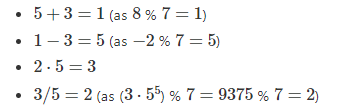
模运算中，分配律仍然成立，即$(a+b)\cdot c=a\cdot c+b\cdot c$成立，甚至$(a^2-b^2)=(a-b)\cdot (a+b)$也仍然成立。

模运算中，除法运算是最难的部分。但是，通过 小费马定理 ，对于任意的非零值 $x<p$，有：
$x^{p-1}\mathrm{m}\mathrm{o}\mathrm{d}p=1$

于是，非零值$x<p$的倒数即为$x^{p-2}=\frac{1}{x}$。
A somewhat more complicated but faster way to evaluate this modular division operator is the extended Euclidean algorithm，implemented in python here。

由于数字是循环的，模运算有时也成为”clock math“：

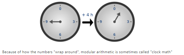
模运算下的系统与传统运算下的系统是自洽的。
密码学家们喜欢使用模运算（又称有限域），是因为 there is a bound on the size of a number that can arise as a result of any modular math calculation - no matter what you do, the values will not “escape” the set { 0 , 1 , 2 , ⋯   , p − 1 } \{0,1,2,\cdots, p-1\} { 0,1,2,⋯,p−1}，即使对100万阶的多项式进行有限域运算，其结果也不超过指定范围。

4. 更实用的举例

将计算转为a set of polynomial equations的更实用的例子为：
已知多项式$P$，在不暴露具体$P(n)$值的情况下，证明$0\le P(n)<2^{64}$。这是blockchain中常用的range proof，用于证明a transaction leaves a balance non-negative without revealing what that balance is。

可借助如下polynomial equations来构建证明：（简单起见，设$n=64$）

• $P(0)=0$
• $P(x+1)=P(x)\ast 2+R(x)$
• R ( x ) ∈ { 0 , 1 } R(x)\in\{0,1\} R(x)∈{ 0,1} across the range { 0 , ⋯   , 63 } \{0,\cdots,63\} { 0,⋯,63}

以上最后两条可再次表述为如下"pure" polynomial equations：【其中$Z(x)=(x-0)\ast (x-1)\ast \cdots \ast (x-63)$】

• $P(x+1)-P(x)\ast 2-R(x)=Z(x)\ast H_1(x)$
• $R(x)\ast (1-R(x))=Z(x)\ast H_2(x)$ 【注意其中的clever trick：$y\ast (1-y)=0$ if and only if y ∈ { 0 , 1 } y\in\{0,1\} y∈{ 0,1}】

核心思想为：
successive evaluations of $P(i)$ build up the number bit-by-bit，即：
若$P(4)=13$，则 the sequence of evaluations going up to that point 可为：
{ 0 , 1 , 3 , 6 , 13 } \{0,1,3,6,13\} { 0,1,3,6,13}。
二进制表示的话，$1$对应为$1$，$3$对应为$11$，$6$对应为$110$，$13$对应为$1101$。
同时$P(x+1)=P(x)\ast 2+R(x)$ keeps adding one bit to the end as long as $R(x)$ is zero or one。

任意的$0\le x<2^{64}$，可通过64步来构建，而任何不再该范围内的数字则不能。

4.1 隐私

以上实现存在一个问题：
How do we know that the commitments to $P(x)$ and $R(x)$ don’t “leak” information that allows us to uncover the exact value of $P(64)$, which we are trying to keep hidden？

好消息是：
以上proofs都是small proofs that can make statements about a large amount of data and computation。因此一般来说，这些proof通常为非常简单而且not be big enough to leak more than a little bit of information。

但是，如何由“only a little bit” 到 “zero”呢？

一种常见的方式是在多项式中加入“fudge factors”，即：
构建$P^{\prime }(x)=P(x)+Z(x)\ast E(x)$ for some random $E(x)$，使得$P^{\prime }$ evaluate to the same values as $P$ on the coordinates that “the computation is happening in”，而加入的噪声$E(x)$可确保$P(x)$的信息不被泄露，从而实现zero knowledge。

在FRI中，需保证sample random points的值不在 { 0 , ⋯   , 64 } \{0,\cdots,64\} { 0,⋯,64}范围内。

迄今为止，扼要概述为：

• 存在3种主流的polynomial commitment scheme，分别为：FRI，Kate和bulletproofs。
• Kate为理论商最容易理解的，但是需要依赖复杂的“black box” of elliptic curve pairings。
• FRI由于仅需依赖hashes，是最酷的：通过逐步reduce a polynomial to a lower and lower-degree polynomial and doing random sample check with Merkle branches to prove equivalence at each step。
• 为了防止数字不断膨胀，将所有的算术运算和多项式运算都基于有限域而不是整数。通常为integers modulo some prime $p$。
• polynomial commitments 自身天然具有隐私保护特性，因其proof远小于多项式本身，因此a polynomial commitment can’t reveal more than a little bit of the information in the polynomial anyway。而通过给多项式加随机值，可实现zero knowledge。

5. 目前进行中的研究

目前进行中的研究方向有：

• 对FRI的优化：通过精心挑选evaluation domains，“DEEP-FRI”，以及借助其它技巧，可提高FRI的效率，Starkware等着力于在这个方向的研究。
• 将计算encode为多项式的方法改进：当前将复杂计算encode为多项式的效率最高的方式主要有：hash函数；memory access等，这些方式都还需要改进。当前最大的改进有 PLOOKUP，但这仍然不够，我们需要更好的方式来实现 encode general-purpose virtual machine execution into polynomials。
• Incrementally verifiable computation：实现了efficiently keep “extending” a proof while a computation continues。在”single-prover”和“multi-prover”场景下均有价值，特别对于blockchain where a different participant creates each block时。具体可看 Halo。

6. 其它研究资料

• Starks：part 1, part 2, part 3
• Specific protocols for encoding computation into polynomials：PLONK
• 其它一些关键的数学优化方法：Fast Fourier transforms
• Starkware在线课程
• Dankrad Feist 的 Kate polynomial commitments 介绍
• bulletproofs polynomial commitment介绍

参考资料

[1] V神博客 An approximate introduction to how zk-SNARKs are possible