3天入门Python机器学习（黑马程序员）

数据集

sklearn
sklearn 包含的内容

sklearn数据集的使用：



以鸢尾花数据集为例：

演示代码如下：

from sklearn.datasets  import load_iris

def datasets_demo():
iris = load_iris()
print(“鸢尾花数据集:\n”,iris)
print(“查看数据集描述:\n”,iris[“DESCR”])
print(“查看特征值的名字:\n”,iris.feature_names)
print(“查看特征值:\n”,iris.data)
print(“查看特征值形状:\n”,iris.data.shape)
return None
if name == “main”:
datasets_demo()

• 1
• 2
• 3
• 4
• 5
• 6
• 7
• 8
• 9
• 10
• 11
• 12

☆这里要注意不要把所有的数据集都拿来训练一个模型，还一个留一部分用来验证，于是有了数据集的划分


以鸢尾花数据集为例代码如下：

from sklearn.datasets  import load_iris
from sklearn.model_selection import train_test_split
def datasets_demo():
    #获取数据集
    iris = load_iris()
    print("鸢尾花数据集:\n",iris)
    print("查看数据集描述:\n",iris["DESCR"])
    print("查看特征值的名字:\n",iris.feature_names)
    print("查看特征值:\n",iris.data)
    print("查看特征值形状:\n",iris.data.shape)
    #数据集的划分
    x_train,x_test,y_train,y_test = train_test_split(iris.data,iris.target,test_size=0.2,random_state=22)
    print("训练集的特征值:\n",x_train,x_train.shape)
    print("测试集的特征值:\n",x_test,x_test.shape)
    return None
if __name__ == "__main__":
    datasets_demo()

 
  
  

 
  
  

   
   
1
   
   
2
   
   
3
   
   
4
   
   
5
   
   
6
   
   
7
   
   
8
   
   
9
   
   
10
   
   
11
   
   
12
   
   
13
   
   
14
   
   
15
   
   
16
   
   
17
  
  

这里我们定义 训练集的特征值（x_train),测试集的特征值（x_test),训练集的目标值（y_train）,测试集的目标值（y_test)

将特征值都处理成one-hot编码

代码如下：

from sklearn.model_selection import train_test_split
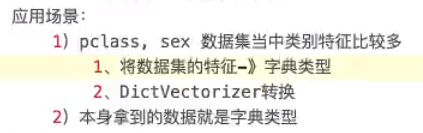
from sklearn.feature_extraction import DictVectorizer

def dict_demo():
data = [{‘city’:‘北京’,‘temperature’:100},{‘city’:‘上海’,‘temperature’:60},{‘city’:‘深圳’,‘temperature’:30}]
#实例一个转换器类
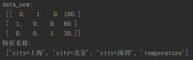
transfer = DictVectorizer(sparse=False)
#调用fit_transform（）
data_new = transfer.fit_transform(data)
print(“data_new:\n”,data_new)
print(“特征名称:\n”,transfer.get_feature_names())
return None

if name== “main”:
dict_demo()

• 1
• 2
• 3
• 4
• 5
• 6
• 7
• 8
• 9
• 10
• 11
• 12
• 13
• 14
• 15

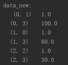
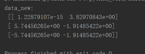
这里可以看到输出并不是我们想象中的二维数组，这是因为当我们实例化DictVectorizer时，他默认有一个参数sparse=True，如果想要得到二维数组形式，需要将sparse=False,但两者应该是等价的，前者对应后者在数组中的位置


例：英文文本分词

from sklearn.model_selection import train_test_split
from sklearn.feature_extraction.text import CountVectorizer

def count_demo():
data = {“Life is short,i like like python”,“Life is too long,i dislike python”}
#实例化一个转化器
transfer = CountVectorizer()
#调用transform
data_new = transfer.fit_transform(data)
print(“data_new:\n”,data_new)
return None
if name == ‘main’:
count_demo()

• 1
• 2
• 3
• 4
• 5
• 6
• 7
• 8
• 9
• 10
• 11
• 12
• 13
• 14

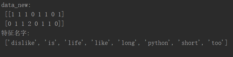
这里我们看到输出又不是我们想要的，这是我想同上面的例子一样在CountVectorizer中加入sparse=False发现行不通，但是sparse矩阵里面有一个默认的方法toarray(),我们可以直接调用这个方法

from sklearn.model_selection import train_test_split
from sklearn.feature_extraction.text import CountVectorizer

def count_demo():
data = {“Life is short,i like like python”,“Life is too long,i dislike python”}
#实例化一个转化器
transfer = CountVectorizer()
#调用transform
data_new = transfer.fit_transform(data)
print(“data_new:\n”,data_new.toarray())
print(“特征名字:\n”,transfer.get_feature_names())
return None
if name == ‘main’:
count_demo()

扫描二维码关注公众号，回复： 11928668 查看本文章

• 1
• 2
• 3
• 4
• 5
• 6
• 7
• 8
• 9
• 10
• 11
• 12
• 13
• 14

这里提到了停用词的概念

例：中文文本分词，需要用到jieba分词

from sklearn.model_selection import train_test_split
from sklearn.feature_extraction.text import CountVectorizer
import jieba

def cut_word(text):
return " ".join(list(jieba.cut(text)))
def count_chinese_demo():
data = {“在北上广深，软考证书可以混个工作居住证，也是一项大的积分落户筹码。”,
“升职加薪必备，很多企业人力资源会以此作为审核晋升的条件。”,
“简历上浓彩重抹一笔，毕竟是国家人力部、工信部承认的IT高级人才。”}
data_new=[]
for sent in data:
data_new.append(cut_word(sent))
#实例化一个转化器
transfer = CountVectorizer()
#调用transform
data_final = transfer.fit_transform(data_new)
print(“data_new:\n”,data_final.toarray())
print(“特征名字:\n”,transfer.get_feature_names())
return None
if name == ‘main’:
count_chinese_demo()

• 1
• 2
• 3
• 4
• 5
• 6
• 7
• 8
• 9
• 10
• 11
• 12
• 13
• 14
• 15
• 16
• 17
• 18
• 19
• 20
• 21
• 22
• 23

但是这种方法也有弊端，于是我们用到了另一种方法





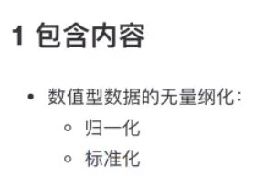
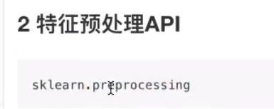
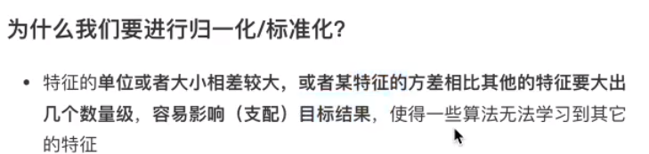
特征预处理就是通过一些转化函数将特征数据转换成更加适合算法模型的特征数据过程（无量纲化处理）





其中[mx-mi]成为区间占比，一般定为0-1

实例：

import pandas as pd
from sklearn.preprocessing import MinMaxScaler
def minmax_demo():
    data = pd.read_csv("dating.txt")
    data = data.iloc[:,:3]  #只取数据前三列
    print("data=\n",data)
    transfer = MinMaxScaler() #默认0-1
    data_new = transfer.fit_transform(data)
    print("data_new=\n",data_new)

if name == ‘main’:
minmax_demo()

• 1
• 2
• 3
• 4
• 5
• 6
• 7
• 8
• 9
• 10
• 11
• 12
• 13

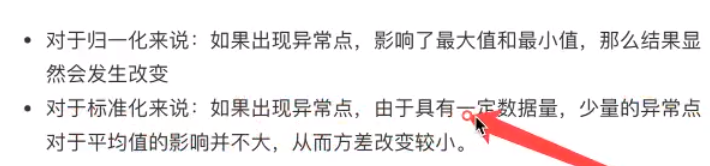
从图中可以看出，如果有异常值对结果的影响并不大


代码与上例类似此处略

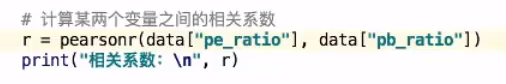
def variance_demo():
    """
    过滤低方差特征
    :return:
    """
    # 1、获取数据
    data = pd.read_csv("factor_returns.csv")
    data = data.iloc[:, 1:-2]
    print("data:\n", data)
# 2、实例化一个转换器类
transfer = VarianceThreshold(threshold=10)

# 3、调用fit_transform
data_new = transfer.fit_transform(data)
print("data_new:\n", data_new, data_new.shape)

# 计算某两个变量之间的相关系数
r1 = pearsonr(data["pe_ratio"], data["pb_ratio"])
print("相关系数：\n", r1)
r2 = pearsonr(data['revenue'], data['total_expense'])
print("revenue与total_expense之间的相关性：\n", r2)

return None

• 1
• 2
• 3
• 4
• 5
• 6
• 7
• 8
• 9
• 10
• 11
• 12
• 13
• 14
• 15
• 16
• 17
• 18
• 19
• 20
• 21
• 22
• 23
• 24
• 25

一个小例子














现在将数据放在一个二维的空间直角坐标系中

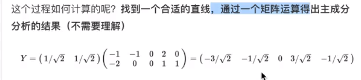
现在我们想办法把二维的数据降成一维（一条直线）

这样我们可以看出，虽然是降成一维，但是由原来的五个点变成三个点，有数据损失了，于是：

由上图我们就可以完成降维的任务了，我们还应该考虑让所有点到直线的距离之和最小。



代码如下：

from sklearn.decomposition  import PCA

def pca_demo():
data = [[2,8,4,5],[6,3,0,8],[5,4,9,1]]
transfer = PCA(n_components=2) #降维成两个特征
data_new = transfer.fit_transform(data)
print(“data_new:\n”,data_new)
return None
if name == ‘main’:
pca_demo()

• 1
• 2
• 3
• 4
• 5
• 6
• 7
• 8
• 9
• 10

这里提到一个instacart案例，有点麻烦这里参考(https://www.bilibili.com/video/av39137333/?p=17)

上文总结

分类算法

其中：





代码如下：

from sklearn.datasets import load_iris
from sklearn.model_selection import  train_test_split
from sklearn.preprocessing import  StandardScaler
from sklearn.neighbors import KNeighborsClassifier

def knn_iris():
#获取数据
iris = load_iris()
#划分数据集
x_train,x_test,y_train,y_test = train_test_split(iris.data,iris.target,random_state=22)
#特征工程:标准化
transfer = StandardScaler()
x_train = transfer.fit_transform(x_train)
x_test = transfer.fit_transform(x_test)
#KNN算法预估器
estimator = KNeighborsClassifier(n_neighbors=3)
estimator.fit(x_train,y_train)
#模型评估
#方法1：直接比对真实值和预测值
y_predict = estimator.predict(x_test)
print(“y_predict:\n”,y_predict)
print(“直接比对真实值和预测值:\n”,y_test == y_predict)
#方法2:计算准确率
score = estimator.score(x_test,y_test)
print(“准确率为:\n”,score)
return None

if name == ‘main’:
knn_iris()

• 1
• 2
• 3
• 4
• 5
• 6
• 7
• 8
• 9
• 10
• 11
• 12
• 13
• 14
• 15
• 16
• 17
• 18
• 19
• 20
• 21
• 22
• 23
• 24
• 25
• 26
• 27
• 28
• 29

![在这里插入图片描述](https://img-blog.csdnimg.cn/20190414205938893.png?x-oss-process=image/watermark,type_ZmFuZ3poZW5naGVpdGk,shadow_10,text_aHR0cHM6Ly9ibG9nLmNzZG4ubmV0L3dlaXhpbl80NDUxNzMwMQ==,size_16,color_FFFFFF,t_70






对鸢尾花数实例进行选择调优

from sklearn.datasets import load_iris
from sklearn.model_selection import  train_test_split
from sklearn.preprocessing import  StandardScaler
from sklearn.neighbors import KNeighborsClassifier
from sklearn.model_selection import GridSearchCV
def knn_iris_gscv():
    #添加网格搜索和交叉验证
    #获取数据
    iris  = load_iris()
    #划分数据集
    x_train,x_test,y_train,y_test = train_test_split(iris.data,iris.target,random_state=22)
    #特征工程:标准化
    transfer = StandardScaler()
    x_train = transfer.fit_transform(x_train)
    x_test = transfer.fit_transform(x_test)
    #KNN算法预估器
    estimator = KNeighborsClassifier() #不用添加k值了
    #网格搜索与交叉验证
    #数据准备
    param_data = {"n_neighbors":[1,3,5,7,9,11]}
    estimator = GridSearchCV(estimator,param_grid=param_data,cv=10)
estimator.fit(x_train,y_train)
#模型评估
#方法1：直接比对真实值和预测值
y_predict = estimator.predict(x_test)
print("y_predict:\n",y_predict)
print("直接比对真实值和预测值:\n",y_test == y_predict)
#方法2:计算准确率
score = estimator.score(x_test,y_test)
print("准确率为:\n",score)
#最佳参数
print("最佳参数:\n",estimator.best_params_)
#最佳结果
print("最佳结果:\n",estimator.best_score_)
#最佳估计器
print("最佳估计器:\n",estimator.best_estimator_)
#交叉验证结果
print("交叉验证结果:\n",estimator.cv_results_)
return None

if name == ‘main’:
knn_iris_gscv()

• 1
• 2
• 3
• 4
• 5
• 6
• 7
• 8
• 9
• 10
• 11
• 12
• 13
• 14
• 15
• 16
• 17
• 18
• 19
• 20
• 21
• 22
• 23
• 24
• 25
• 26
• 27
• 28
• 29
• 30
• 31
• 32
• 33
• 34
• 35
• 36
• 37
• 38
• 39
• 40
• 41
• 42
• 43

一个比较大的实例：预测facebook签到位置有点难啊嗷嗷嗷

import pandas as pd
from sklearn.model_selection import train_test_split
from sklearn.preprocessing import StandardScaler
from sklearn.neighbors import KNeighborsClassifier
from sklearn.model_selection import GridSearchCV

def facebook_demo():
data = pd.read_csv(“F:/python_work/train.csv”)

#缩小数据范围
data = data.query("x<2.5 & x>2 & y<1.5 & y>1")

#处理时间特征
#转换为年月日时分秒
time_value = pd.to_datetime(data["time"],unit="s")
date = pd.DatetimeIndex(time_value)
#人工排除年和月两个信息
data["day"] = date.day
data["weekday"] = date.weekday
data["hour"] = date.hour
print(data)
#过滤掉签到次数少的地方
#先统计每个地点被签到的次数
place_count = data.groupby("place_id").count()[ "row_id"]
place_count[place_count>3]
data_final=data[data["place_id"].isin(place_count[place_count>3].index.values)]
# 筛选特征值和目标值
x = data_final[["x", "y", "accuracy", "day", "weekday", "hour"]]
y = data_final["place_id"]
# 数据集划分
x_train, x_test, y_train, y_test = train_test_split(x, y)
# 3）特征工程：标准化
transfer = StandardScaler()
x_train = transfer.fit_transform(x_train)
x_test = transfer.transform(x_test)

# 4）KNN算法预估器
estimator = KNeighborsClassifier()

# 加入网格搜索与交叉验证
# 参数准备
param_dict = {"n_neighbors": [3, 5, 7, 9]}
estimator = GridSearchCV(estimator, param_grid=param_dict, cv=3)
estimator.fit(x_train, y_train)
# 5）模型评估
# 方法1：直接比对真实值和预测值
y_predict = estimator.predict(x_test)
print("y_predict:\n", y_predict)
print("直接比对真实值和预测值:\n", y_test == y_predict)

# 方法2：计算准确率
score = estimator.score(x_test, y_test)
print("准确率为：\n", score)

# 最佳参数：best_params_
print("最佳参数：\n", estimator.best_params_)
# 最佳结果：best_score_
print("最佳结果：\n", estimator.best_score_)
# 最佳估计器：best_estimator_
print("最佳估计器:\n", estimator.best_estimator_)
# 交叉验证结果：cv_results_
print("交叉验证结果:\n", estimator.cv_results_)

if name == ‘main’:
facebook_demo()

• 1
• 2
• 3
• 4
• 5
• 6
• 7
• 8
• 9
• 10
• 11
• 12
• 13
• 14
• 15
• 16
• 17
• 18
• 19
• 20
• 21
• 22
• 23
• 24
• 25
• 26
• 27
• 28
• 29
• 30
• 31
• 32
• 33
• 34
• 35
• 36
• 37
• 38
• 39
• 40
• 41
• 42
• 43
• 44
• 45
• 46
• 47
• 48
• 49
• 50
• 51
• 52
• 53
• 54
• 55
• 56
• 57
• 58
• 59
• 60
• 61
• 62
• 63
• 64

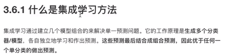
朴素贝叶斯算法原理(假设特征与特征之间的相互独立的）

在这里我们计算出p(Tokyo|C)=0；

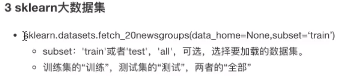
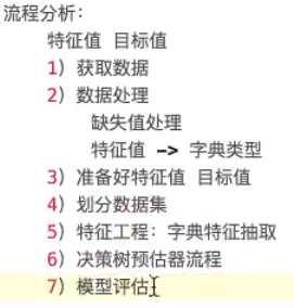
from sklearn.datasets import fetch_20newsgroups
from sklearn.model_selection import train_test_split
from sklearn.feature_extraction.text import TfidfVectorizer
from sklearn.naive_bayes import MultinomialNB
def nb_news():
    """
    用朴素贝叶斯算法对新闻进行分类
    :return:
    """
    # 1）获取数据
    news = fetch_20newsgroups(subset="all")
# 2）划分数据集
x_train, x_test, y_train, y_test = train_test_split(news.data, news.target)

# 3）特征工程：文本特征抽取-tfidf
transfer = TfidfVectorizer()
x_train = transfer.fit_transform(x_train)
x_test = transfer.transform(x_test)

# 4）朴素贝叶斯算法预估器流程
estimator = MultinomialNB()
estimator.fit(x_train, y_train)

# 5）模型评估
# 方法1：直接比对真实值和预测值
y_predict = estimator.predict(x_test)
print("y_predict:\n", y_predict)
print("直接比对真实值和预测值:\n", y_test == y_predict)

# 方法2：计算准确率
score = estimator.score(x_test, y_test)
print("准确率为：\n", score)

return None

if name == ‘main’:
nb_news()

• 1
• 2
• 3
• 4
• 5
• 6
• 7
• 8
• 9
• 10
• 11
• 12
• 13
• 14
• 15
• 16
• 17
• 18
• 19
• 20
• 21
• 22
• 23
• 24
• 25
• 26
• 27
• 28
• 29
• 30
• 31
• 32
• 33
• 34
• 35
• 36
• 37
• 38

决策树

例：





以鸢尾花数据集为例实现决策树

from sklearn.datasets import load_iris
from sklearn.model_selection import train_test_split
from sklearn.tree import DecisionTreeClassifier, export_graphviz
def decision_iris():
    """
    用决策树对鸢尾花进行分类
    :return:
    """
    # 1）获取数据集
    iris = load_iris()
# 2）划分数据集
x_train, x_test, y_train, y_test = train_test_split(iris.data, iris.target, random_state=22)

# 3）决策树预估器
estimator = DecisionTreeClassifier(criterion="entropy")
estimator.fit(x_train, y_train)

# 4）模型评估
# 方法1：直接比对真实值和预测值
y_predict = estimator.predict(x_test)
print("y_predict:\n", y_predict)
print("直接比对真实值和预测值:\n", y_test == y_predict)

# 方法2：计算准确率
score = estimator.score(x_test, y_test)
print("准确率为：\n", score)

# 可视化决策树
export_graphviz(estimator, out_file="iris_tree.dot", feature_names=iris.feature_names)

return None

if name == ‘main’:
decision_iris()

• 1
• 2
• 3
• 4
• 5
• 6
• 7
• 8
• 9
• 10
• 11
• 12
• 13
• 14
• 15
• 16
• 17
• 18
• 19
• 20
• 21
• 22
• 23
• 24
• 25
• 26
• 27
• 28
• 29
• 30
• 31
• 32
• 33
• 34

这时，文件里的内容我们还是看不懂的，于是我们需要把内容放到一个生成树的网站里
(https://webgraphviz.com/)

点击网站最下面的


用决策树实现泰坦尼克号乘客生存预测


代码：

import pandas as pd
from sklearn.model_selection import train_test_split
from sklearn.feature_extraction import DictVectorizer
from sklearn.tree import DecisionTreeClassifier, export_graphviz
def titanic():
    # 1、获取数据
    path = "http://biostat.mc.vanderbilt.edu/wiki/pub/Main/DataSets/titanic.txt"
    titanic = pd.read_csv(path)
    # 筛选特征值和目标值
    x = titanic[["pclass", "age", "sex"]]
    y = titanic["survived"]
    # 2、数据处理
    # 1）缺失值处理
    x["age"].fillna(x["age"].mean(), inplace=True) #填充平均值
    # 2) 转换成字典
    x = x.to_dict(orient="records")
    # 3、数据集划分
    x_train, x_test, y_train, y_test = train_test_split(x, y, random_state=22)
    # 4、字典特征抽取
    transfer = DictVectorizer()
    x_train = transfer.fit_transform(x_train)
    x_test = transfer.transform(x_test)
    # 3）决策树预估器
    estimator = DecisionTreeClassifier(criterion="entropy", max_depth=8)
    estimator.fit(x_train, y_train)
# 4）模型评估
# 方法1：直接比对真实值和预测值
y_predict = estimator.predict(x_test)
print("y_predict:\n", y_predict)
print("直接比对真实值和预测值:\n", y_test == y_predict)

# 方法2：计算准确率
score = estimator.score(x_test, y_test)
print("准确率为：\n", score)

# 可视化决策树
export_graphviz(estimator, out_file="titanic_tree.dot", feature_names=transfer.get_feature_names())

if name == ‘main’:
titanic()

• 1
• 2
• 3
• 4
• 5
• 6
• 7
• 8
• 9
• 10
• 11
• 12
• 13
• 14
• 15
• 16
• 17
• 18
• 19
• 20
• 21
• 22
• 23
• 24
• 25
• 26
• 27
• 28
• 29
• 30
• 31
• 32
• 33
• 34
• 35
• 36
• 37
• 38
• 39
• 40

随机森林

用随机森林实现泰坦尼克号实例

from sklearn.ensemble import RandomForestClassifier
from sklearn.model_selection import GridSearchCV
from sklearn.model_selection import train_test_split
import pandas as pd
from sklearn.feature_extraction import DictVectorizer
def suijisanli_demo():
    # 1、获取数据
    path = "http://biostat.mc.vanderbilt.edu/wiki/pub/Main/DataSets/titanic.txt"
    titanic = pd.read_csv(path)
    # 筛选特征值和目标值
    x = titanic[["pclass", "age", "sex"]]
    y = titanic["survived"]
    # 2、数据处理
    # 1）缺失值处理
    x["age"].fillna(x["age"].mean(), inplace=True)
    # 2) 转换成字典
    x = x.to_dict(orient="records")
    # 3、数据集划分
    x_train, x_test, y_train, y_test = train_test_split(x, y, random_state=22)
    # 4、字典特征抽取
    transfer = DictVectorizer()
    x_train = transfer.fit_transform(x_train)
    x_test = transfer.transform(x_test)
    #随机森林预估器
    estimator = RandomForestClassifier()
    # 加入网格搜索与交叉验证
    # 参数准备
    param_dict = {"n_estimators": [120, 200, 300, 500, 800, 1200], "max_depth": [5, 8, 15, 25, 30]}
    estimator = GridSearchCV(estimator, param_grid=param_dict, cv=3)
    estimator.fit(x_train, y_train)
# 5）模型评估
# 方法1：直接比对真实值和预测值
y_predict = estimator.predict(x_test)
print("y_predict:\n", y_predict)
print("直接比对真实值和预测值:\n", y_test == y_predict)

# 方法2：计算准确率
score = estimator.score(x_test, y_test)
print("准确率为：\n", score)

# 最佳参数：best_params_
print("最佳参数：\n", estimator.best_params_)
# 最佳结果：best_score_
print("最佳结果：\n", estimator.best_score_)
# 最佳估计器：best_estimator_
print("最佳估计器:\n", estimator.best_estimator_)
# 交叉验证结果：cv_results_
print("交叉验证结果:\n", estimator.cv_results_)

if name == ‘main’:
suijisanli_demo()

• 1
• 2
• 3
• 4
• 5
• 6
• 7
• 8
• 9
• 10
• 11
• 12
• 13
• 14
• 15
• 16
• 17
• 18
• 19
• 20
• 21
• 22
• 23
• 24
• 25
• 26
• 27
• 28
• 29
• 30
• 31
• 32
• 33
• 34
• 35
• 36
• 37
• 38
• 39
• 40
• 41
• 42
• 43
• 44
• 45
• 46
• 47
• 48
• 49
• 50
• 51
• 52

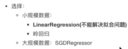
回归与聚类算法

注：线性关系一定是线性模型，线性模型不一定是线性关系


即：目标就是找到一条直线，使所有点到直线的距离之和最小，即误差最小

优化方法一、正规方程

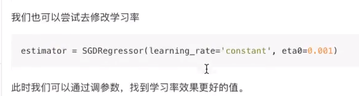
优化方法二、梯度下降







代码如下：

from sklearn.datasets import load_boston
from sklearn.model_selection import train_test_split
from sklearn.preprocessing import StandardScaler
from sklearn.linear_model import LinearRegression, SGDRegressor
from sklearn.metrics import mean_squared_error
def linear1():
    """
    正规方程的优化方法对波士顿房价进行预测
    :return:
    """
    # 1）获取数据
    boston = load_boston()
# 2）划分数据集
x_train, x_test, y_train, y_test = train_test_split(boston.data, boston.target, random_state=22)

# 3）标准化
transfer = StandardScaler()
x_train = transfer.fit_transform(x_train)
x_test = transfer.transform(x_test)

# 4）预估器
estimator = LinearRegression()
estimator.fit(x_train, y_train)

# 5）得出模型
print("正规方程-权重系数为：\n", estimator.coef_)
print("正规方程-偏置为：\n", estimator.intercept_)

# 6）模型评估
y_predict = estimator.predict(x_test)
print("预测房价：\n", y_predict)
error = mean_squared_error(y_test, y_predict)
print("正规方程-均方误差为：\n", error)

return None

def linear2():
“”"
梯度下降的优化方法对波士顿房价进行预测
:return:
“”"
# 1）获取数据
boston = load_boston()
print(“特征数量：\n”, boston.data.shape)

# 2）划分数据集
x_train, x_test, y_train, y_test = train_test_split(boston.data, boston.target, random_state=22)

# 3）标准化
transfer = StandardScaler()
x_train = transfer.fit_transform(x_train)
x_test = transfer.transform(x_test)

# 4）预估器
estimator = SGDRegressor(learning_rate="constant", eta0=0.01, max_iter=10000, penalty="l1")
estimator.fit(x_train, y_train)

# 5）得出模型
print("梯度下降-权重系数为：\n", estimator.coef_)
print("梯度下降-偏置为：\n", estimator.intercept_)

# 6）模型评估
y_predict = estimator.predict(x_test)
print("预测房价：\n", y_predict)
error = mean_squared_error(y_test, y_predict)
print("梯度下降-均方误差为：\n", error)

return None

if name == ‘main’:
linear1()
linear2()

• 1
• 2
• 3
• 4
• 5
• 6
• 7
• 8
• 9
• 10
• 11
• 12
• 13
• 14
• 15
• 16
• 17
• 18
• 19
• 20
• 21
• 22
• 23
• 24
• 25
• 26
• 27
• 28
• 29
• 30
• 31
• 32
• 33
• 34
• 35
• 36
• 37
• 38
• 39
• 40
• 41
• 42
• 43
• 44
• 45
• 46
• 47
• 48
• 49
• 50
• 51
• 52
• 53
• 54
• 55
• 56
• 57
• 58
• 59
• 60
• 61
• 62
• 63
• 64
• 65
• 66
• 67
• 68
• 69
• 70
• 71
• 72
• 73
• 74

两种方法的对比




以计算机识别天鹅为例，第一种欠拟合，第二种过拟合





hw(xi)为预测值，yi为真实值，L1正则化就是把wj²改为|wj|

from sklearn.datasets import load_boston
from sklearn.model_selection import train_test_split
from sklearn.preprocessing import StandardScaler
from sklearn.linear_model import LinearRegression, SGDRegressor,Ridge
from sklearn.metrics import mean_squared_error

def linear3():
“”"
岭回归对波士顿房价进行预测
:return:
“”"
# 1）获取数据
boston = load_boston()
print(“特征数量：\n”, boston.data.shape)

# 2）划分数据集
x_train, x_test, y_train, y_test = train_test_split(boston.data, boston.target, random_state=22)

# 3）标准化
transfer = StandardScaler()
x_train = transfer.fit_transform(x_train)
x_test = transfer.transform(x_test)

#4）预估器
estimator = Ridge(alpha=0.5, max_iter=10000)
estimator.fit(x_train, y_train)


# 5）得出模型
print("岭回归-权重系数为：\n", estimator.coef_)
print("岭回归-偏置为：\n", estimator.intercept_)

# 6）模型评估
y_predict = estimator.predict(x_test)
print("预测房价：\n", y_predict)
error = mean_squared_error(y_test, y_predict)
print("岭回归-均方误差为：\n", error)

return None

if name == ‘main’:
linear3()

• 1
• 2
• 3
• 4
• 5
• 6
• 7
• 8
• 9
• 10
• 11
• 12
• 13
• 14
• 15
• 16
• 17
• 18
• 19
• 20
• 21
• 22
• 23
• 24
• 25
• 26
• 27
• 28
• 29
• 30
• 31
• 32
• 33
• 34
• 35
• 36
• 37
• 38
• 39
• 40
• 41

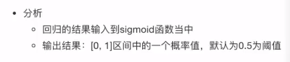
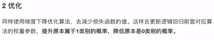
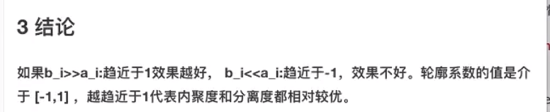
总结：

from sklearn.model_selection import train_test_split
from sklearn.preprocessing import StandardScaler
from sklearn.linear_model import LogisticRegression
import pandas as pd
import numpy as np

def cancer():
# 1、读取数据
path = “https://archive.ics.uci.edu/ml/machine-learning-databases/breast-cancer-wisconsin/breast-cancer-wisconsin.data”
column_name = [‘Sample code number’, ‘Clump Thickness’, ‘Uniformity of Cell Size’, ‘Uniformity of Cell Shape’,
‘Marginal Adhesion’, ‘Single Epithelial Cell Size’, ‘Bare Nuclei’, ‘Bland Chromatin’,
‘Normal Nucleoli’, ‘Mitoses’, ‘Class’]

data = pd.read_csv(path, names=column_name)
# 2、缺失值处理
# 1）替换-》np.nan
data = data.replace(to_replace="?", value=np.nan)
# 2）删除缺失样本
data.dropna(inplace=True)
data.isnull().any()  # 检验,不存在缺失值
# 3、划分数据集
# 筛选特征值和目标值
x = data.iloc[:, 1:-1]
y = data["Class"]
x_train, x_test, y_train, y_test = train_test_split(x, y)
# 4、标准化
transfer = StandardScaler()
x_train = transfer.fit_transform(x_train)
x_test = transfer.transform(x_test)
# 5、预估器流程
estimator = LogisticRegression()
estimator.fit(x_train, y_train)
# 5）得出模型
print("逻辑回归-权重系数为：\n", estimator.coef_)
print("逻辑回归-偏置为：\n", estimator.intercept_)
# 6、模型评估
# 方法1：直接比对真实值和预测值
y_predict = estimator.predict(x_test)
print("y_predict:\n", y_predict)
print("直接比对真实值和预测值:\n", y_test == y_predict)

# 方法2：计算准确率
score = estimator.score(x_test, y_test)
print("准确率为：\n", score)

if name == ‘main’:
cancer()

• 1
• 2
• 3
• 4
• 5
• 6
• 7
• 8
• 9
• 10
• 11
• 12
• 13
• 14
• 15
• 16
• 17
• 18
• 19
• 20
• 21
• 22
• 23
• 24
• 25
• 26
• 27
• 28
• 29
• 30
• 31
• 32
• 33
• 34
• 35
• 36
• 37
• 38
• 39
• 40
• 41
• 42
• 43
• 44
• 45
• 46
• 47

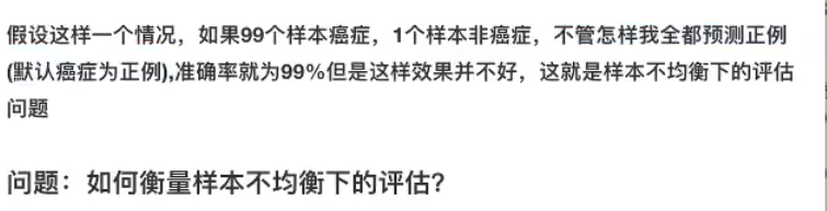
from sklearn.model_selection import train_test_split
from sklearn.preprocessing import StandardScaler
from sklearn.linear_model import LogisticRegression
import pandas as pd
import numpy as np
from sklearn.metrics import classification_report
from sklearn.metrics import roc_auc_score
def cancer():
    # 1、读取数据
    path = "https://archive.ics.uci.edu/ml/machine-learning-databases/breast-cancer-wisconsin/breast-cancer-wisconsin.data"
    column_name = ['Sample code number', 'Clump Thickness', 'Uniformity of Cell Size', 'Uniformity of Cell Shape',
                   'Marginal Adhesion', 'Single Epithelial Cell Size', 'Bare Nuclei', 'Bland Chromatin',
                   'Normal Nucleoli', 'Mitoses', 'Class']
data = pd.read_csv(path, names=column_name)
# 2、缺失值处理
# 1）替换-》np.nan
data = data.replace(to_replace="?", value=np.nan)
# 2）删除缺失样本
data.dropna(inplace=True)
data.isnull().any()  # 检验,不存在缺失值
# 3、划分数据集
# 筛选特征值和目标值
x = data.iloc[:, 1:-1]
y = data["Class"]
x_train, x_test, y_train, y_test = train_test_split(x, y)
# 4、标准化
transfer = StandardScaler()
x_train = transfer.fit_transform(x_train)
x_test = transfer.transform(x_test)
# 5、预估器流程
estimator = LogisticRegression()
estimator.fit(x_train, y_train)
# 5）得出模型
print("逻辑回归-权重系数为：\n", estimator.coef_)
print("逻辑回归-偏置为：\n", estimator.intercept_)
# 6、模型评估
# 方法1：直接比对真实值和预测值
y_predict = estimator.predict(x_test)
print("y_predict:\n", y_predict)
print("直接比对真实值和预测值:\n", y_test == y_predict)

# 方法2：计算准确率
score = estimator.score(x_test, y_test)
print("准确率为：\n", score)
# 查看精确率、召回率、F1-score
report = classification_report(y_test, y_predict, labels=[2, 4], target_names=["良性", "恶性"])
print(report)
# y_true：每个样本的真实类别，必须为0(反例),1(正例)标记
# 将y_test 转换成 0 1
y_true = np.where(y_test > 3, 1, 0)
score = roc_auc_score(y_true, y_predict)
print(score)

if name == ‘main’:
cancer()

• 1
• 2
• 3
• 4
• 5
• 6
• 7
• 8
• 9
• 10
• 11
• 12
• 13
• 14
• 15
• 16
• 17
• 18
• 19
• 20
• 21
• 22
• 23
• 24
• 25
• 26
• 27
• 28
• 29
• 30
• 31
• 32
• 33
• 34
• 35
• 36
• 37
• 38
• 39
• 40
• 41
• 42
• 43
• 44
• 45
• 46
• 47
• 48
• 49
• 50
• 51
• 52
• 53
• 54
• 55

import pandas as pd
from sklearn.decomposition import PCA
from sklearn.cluster import KMeans
from sklearn.metrics import silhouette_score

def lunkuoxishu():
# 1、获取数据
order_products = pd.read_csv("./instacart/order_products__prior.csv")
products = pd.read_csv("./instacart/products.csv")
orders = pd.read_csv("./instacart/orders.csv")
aisles = pd.read_csv("./instacart/aisles.csv")
# 2、合并表
# order_products__prior.csv：订单与商品信息

# 字段：order_id, product_id, add_to_cart_order, reordered
# products.csv：商品信息
# 字段：product_id, product_name, aisle_id, department_id
# orders.csv：用户的订单信息
# 字段：order_id,user_id,eval_set,order_number,….
# aisles.csv：商品所属具体物品类别
# 字段： aisle_id, aisle

# 合并aisles和products aisle和product_id
tab1 = pd.merge(aisles, products, on=["aisle_id", "aisle_id"])
tab2 = pd.merge(tab1, order_products, on=["product_id", "product_id"])
tab3 = pd.merge(tab2, orders, on=["order_id", "order_id"])
# 3、找到user_id和aisle之间的关系
table = pd.crosstab(tab3["user_id"], tab3["aisle"])
data = table[:10000]
# 4、PCA降维
# 1）实例化一个转换器类
transfer = PCA(n_components=0.95)

# 2）调用fit_transform
data_new = transfer.fit_transform(data)
data_new.shape
# 预估器流程
estimator = KMeans(n_clusters=3)
estimator.fit(data_new)
y_predict = estimator.predict(data_new)
y_predict[:300]
# 模型评估-轮廓系数
silhouette_score(data_new, y_predict)

if name == ‘main’:
lunkuoxishu()

• 1
• 2
• 3
• 4
• 5
• 6
• 7
• 8
• 9
• 10
• 11
• 12
• 13
• 14
• 15
• 16
• 17
• 18
• 19
• 20
• 21
• 22
• 23
• 24
• 25
• 26
• 27
• 28
• 29
• 30
• 31
• 32
• 33
• 34
• 35
• 36
• 37
• 38
• 39
• 40
• 41
• 42
• 43
• 44
• 45
• 46

**参考：**https://blog.csdn.net/weixin_44517301/article/details/88405939