无人驾驶汽车系统入门(二十七)——基于地面平面拟合的激光雷达地面分割方法和ROS实现
在博客的第二十四篇中,我们介绍了一种基于射线的地面过滤方法,此方法能够很好的完成地面分割,但是存在几点不足:第一,存在少量噪点,不能彻底过滤出地面;第二,非地面的点容易被错误分类,造成非地面点缺失;第三,对于目标接近激光雷达盲区的情况,会出现误分割,即将非地面点云分割为地面。通过本文我们一起学习一种新的地面分割方法,出自论文:Fast segmentation of 3D point clouds: A paradigm on LiDAR data for autonomous vehicle applications,在可靠性、分割精度方面均优于基于射线的地面分割方法。我们将其称之为地面平面拟合方法。
地面平面拟合(Ground Plane Fitting)
我们采用平面模型(Plane Model)来拟合当前的地面,通常来说,由于现实的地面并不是一个“完美的”平面,而且当距离较大时激光雷达会存在一定的测量噪声,单一的平面模型并不足以描述我们现实的地面。要很好的完成地面分割,就必须要处理存在一定坡度变化的地面的情况(不能将这种坡度的变化视为非地面,不能因为坡度的存在而引入噪声),一种简单的处理方法就是沿着x方向(车头的方向)将空间分割成若干个子平面,然后对每个子平面使用地面平面拟合算法(GPF)从而得到能够处理陡坡的地面分割方法。
那么如何进行平面拟合呢?其伪代码如下:
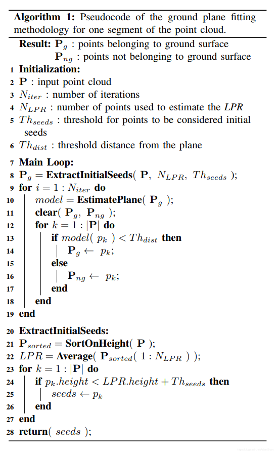
我们来详细的了解这一流程:对于给定的点云 ,分割的最终结果为两个点云集合 :地面点云 和 :非地面点云。该算法有四个重要的参数,分别是:
- : 进行奇异值分解(singular value decomposition,SVD)的次数,也即进行优化拟合的次数
- : 用于选取LPR的最低高度点的数量
- : 用于选取种子点的阈值,当点云内的点的高度小于LPR的高度加上此阈值时,我们将该点加入种子点集
- : 平面距离阈值,我们会计算点云中每一个点到我们拟合的平面的正交投影的距离,而这个平面距离阈值,就是用来判定点是否属于地面
种子点集的选取
我们首先选取一个种子点集(seed point set),这些种子点来源于点云中高度(即z值)较小的点,种子点集被用于建立描述地面的初始平面模型,那么如何选取这个种子点集呢?我们引入最低点代表(Lowest Point Representative, LPR)的概念。LPR就是 个最低高度点的平均值,LPR保证了平面拟合阶段不受测量噪声的影响。这个LPR被当作是整个点云 的最低点,点云P中高度在阈值 内的点被当作是种子点,由这些种子点构成一个种子点集合。
种子点集的选取代码如下:
/*
    @brief Extract initial seeds of the given pointcloud sorted segment.
    This function filter ground seeds points accoring to heigt.
    This function will set the `g_ground_pc` to `g_seed_pc`.
    @param p_sorted: sorted pointcloud

    @param ::num_lpr_: num of LPR points
    @param ::th_seeds_: threshold distance of seeds
    @param ::
*/
void PlaneGroundFilter::extract_initial_seeds_(const pcl::PointCloud<VPoint> &p_sorted)
{
    // LPR is the mean of low point representative
    double sum = 0;
    int cnt = 0;
    // Calculate the mean height value.
    for (int i = 0; i < p_sorted.points.size() && cnt < num_lpr_; i++)
    {
        sum += p_sorted.points[i].z;
        cnt++;
    }
    double lpr_height = cnt != 0 ? sum / cnt : 0; // in case divide by 0
    g_seeds_pc->clear();
    // iterate pointcloud, filter those height is less than lpr.height+th_seeds_
    for (int i = 0; i < p_sorted.points.size(); i++)
    {
        if (p_sorted.points[i].z < lpr_height + th_seeds_)
        {
            g_seeds_pc->points.push_back(p_sorted.points[i]);
        }
    }
    // return seeds points
}
输入是一个点云,这个点云内的点已经沿着z方向(即高度)做了排序,取 num_lpr_ 个最小点,求得高度平均值 lpr_height(即LPR),选取高度小于 lpr_height + th_seeds_的点作为种子点。
平面模型
接下来我们需要确定一个平面,点云中的点到这个平面的正交投影距离小于阈值 则认为该点属于地面,否则属于非地面,我们采用一个简单的线性模型用于平面模型估计,如下:
也即:
其中 , ,通过初始点集的协方差矩阵 来求解 (即a, b, c), 从而确定一个平面, 我们采用种子点集 作为初始点集,其协方差矩阵为:
其中, 是所有点的均值。这个协方差矩阵 描述了种子点集的散布情况,其三个奇异向量可以通过奇异值分解(Singular Value Decomposition,SVD)求得,这三个奇异向量描述了点集在三个主要方向的散布情况。由于是平面模型,垂直于平面的法向量 表示具有最小方差的方向,可以通过计算具有最小奇异值的奇异向量来求得。
那么在求得了 以后, 可以通过代入种子点集的平均值 (它代表属于地面的点) 直接求得。整个平面模型计算代码如下:
/*
    @brief The function to estimate plane model. The
    model parameter `normal_` and `d_`, and `th_dist_d_`
    is set here.
    The main step is performed SVD(UAV) on covariance matrix.
    Taking the sigular vector in U matrix according to the smallest
    sigular value in A, as the `normal_`. `d_` is then calculated
    according to mean ground points.

    @param g_ground_pc:global ground pointcloud ptr.

*/
void PlaneGroundFilter::estimate_plane_(void)
{
    // Create covarian matrix in single pass.
    // TODO: compare the efficiency.
    Eigen::Matrix3f cov;
    Eigen::Vector4f pc_mean;
    pcl::computeMeanAndCovarianceMatrix(*g_ground_pc, cov, pc_mean);
    // Singular Value Decomposition: SVD
    JacobiSVD<MatrixXf> svd(cov, Eigen::DecompositionOptions::ComputeFullU);
    // use the least singular vector as normal
    normal_ = (svd.matrixU().col(2));
    // mean ground seeds value
    Eigen::Vector3f seeds_mean = pc_mean.head<3>();

    // according to normal.T*[x,y,z] = -d
    d_ = -(normal_.transpose() * seeds_mean)(0, 0);
    // set distance threhold to `th_dist - d`
    th_dist_d_ = th_dist_ - d_;

    // return the equation parameters
}
优化平面主循环
在确定如何选取种子点集以及如何估计平面模型以后,我们来看一下整个算法的主循环,以下是主循环的代码:
extract_initial_seeds_(laserCloudIn);
g_ground_pc = g_seeds_pc;
// Ground plane fitter mainloop
for (int i = 0; i < num_iter_; i++)
{
    estimate_plane_();
    g_ground_pc->clear();
    g_not_ground_pc->clear();

    //pointcloud to matrix
    MatrixXf points(laserCloudIn_org.points.size(), 3);
    int j = 0;
    for (auto p : laserCloudIn_org.points)
    {
        points.row(j++) << p.x, p.y, p.z;
    }
    // ground plane model
    VectorXf result = points * normal_;
    // threshold filter
    for (int r = 0; r < result.rows(); r++)
    {
        if (result[r] < th_dist_d_)
        {
            g_all_pc->points[r].label = 1u; // means ground
            g_ground_pc->points.push_back(laserCloudIn_org[r]);
        }
        else
        {
            g_all_pc->points[r].label = 0u; // means not ground and non clusterred
            g_not_ground_pc->points.push_back(laserCloudIn_org[r]);
        }
    }
}
得到这个初始的平面模型以后,我们会计算点云中每一个点到该平面的正交投影的距离,即 points * normal_,并且将这个距离与设定的阈值
(即th_dist_d_) 比较,当高度差小于此阈值,我们认为该点属于地面,当高度差大于此阈值,则为非地面点。经过分类以后的所有地面点被当作下一次迭代的种子点集,迭代优化。
ROS实践
下面我们编写一个简单的ROS节点实现这一地面分割算法。我们仍然采用第24篇博客(激光雷达的地面-非地面分割和pcl_ros实践)中的bag进行实验,这个bag来自Velodyne的VLP32C,在此算法的基础上我们要进一步滤除雷达过近处和过高处的点,因为雷达安装位置的原因,近处的车身反射会对Detection造成影响,需要滤除; 过高的目标,如大树、高楼,对于无人车的雷达感知意义也不大,我们对过近过高的点进行切除,代码如下:
void PlaneGroundFilter::clip_above(const pcl::PointCloud<VPoint>::Ptr in,
                                   const pcl::PointCloud<VPoint>::Ptr out)
{
    pcl::ExtractIndices<VPoint> cliper;

    cliper.setInputCloud(in);
    pcl::PointIndices indices;
#pragma omp for
    for (size_t i = 0; i < in->points.size(); i++)
    {
        if (in->points[i].z > clip_height_)
        {
            indices.indices.push_back(i);
        }
    }
    cliper.setIndices(boost::make_shared<pcl::PointIndices>(indices));
    cliper.setNegative(true); //ture to remove the indices
    cliper.filter(*out);
}

void PlaneGroundFilter::remove_close_far_pt(const pcl::PointCloud<VPoint>::Ptr in,
                                            const pcl::PointCloud<VPoint>::Ptr out)
{
    pcl::ExtractIndices<VPoint> cliper;

    cliper.setInputCloud(in);
    pcl::PointIndices indices;
#pragma omp for
    for (size_t i = 0; i < in->points.size(); i++)
    {
        double distance = sqrt(in->points[i].x * in->points[i].x + in->points[i].y * in->points[i].y);

        if ((distance < min_distance_) || (distance > max_distance_))
        {
            indices.indices.push_back(i);
        }
    }
    cliper.setIndices(boost::make_shared<pcl::PointIndices>(indices));
    cliper.setNegative(true); //ture to remove the indices
    cliper.filter(*out);
}
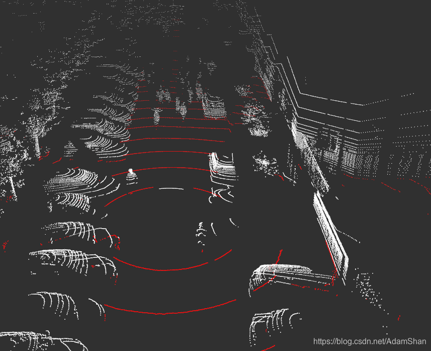
编译并运行该ROS节点,使用我们在第二十四篇博客中提供的bag进行测试,得到如下结果: