如何基于DCGAN网络模型使用tensorflow生成仿真的人脸图像?(CelebA数据集)
文章目录
- 如何基于DCGAN网络模型使用tensorflow生成仿真的人脸图像?(CelebA数据集)
- 1.GAN网络模型的设计思想?
- 2.数据集的准备?
- 3.如何一步一步构建我们的人脸fake模型?
- 1.相关库的导入。
- 2.设置训练图片数据集路径,拿到图片数量。设置好batch_size(读取数据的批次大小),z_dim(fake图片的原始随机点,后经过生成器(Generator)生成fake图片。),输入图片的宽和高,以及输出路径。
- 3.设置X(输入量),noise(随机噪声), is_training(是否进行训练,便于模型的保存和加载)的变量格式。
- 4.定义相关的激活函数,损失函数。
- 5.定义判别器(Discriminator)的网络结构。
- 6.定义生成器(Generator)的网络结构:
- 7.得到fake的假人脸图片,==经判别器映射之后的输入图片,未经sigmoid激活的输入图片的输出层数据,以及返回generator,discriminator中所有可训练的变量。==
- 8.定义生成器和判别器的Loss函数。
- 9.定义更新训练操作:
- 10.定义读取图片函数:
- 11.定义合并fake图片的函数:
- 12.定义session(),fake的原始随机点,loss以及samples。
- 13.写for in in range( )大循环,进行迭代训练。
- 14.保存模型
- 15.训练过程的GIF动态展示
1.GAN网络模型的设计思想?
GAN中的核心网络结构:
- 生成器(Generator):记作G,通过对大量样本的学习,能生成一些以假乱真的样本。
- 判别器(Discriminator):记作D,接受真实样本和G生成的样本,并进行判别和区分。
- G和D相互博弈,通过学习,G的生成能力和D的判别能力都逐渐增强并收敛。
【注】:GAN在实际的训练中,有很多苛刻的细节要求需要注意。
2.数据集的准备?
CelebA人脸图片数据集,共202599张人脸图片,图片的宽高比=178:218。(本文涉及的数据集与代码均已上传,链接提取密码:21re)
3.如何一步一步构建我们的人脸fake模型?
1.相关库的导入。
import tensorflow as tf
import numpy as np
import os
from imageio import imread, imsave
import cv2
import glob
2.设置训练图片数据集路径,拿到图片数量。设置好batch_size(读取数据的批次大小),z_dim(fake图片的原始随机点,后经过生成器(Generator)生成fake图片。),输入图片的宽和高,以及输出路径。
dataset = 'celeba'  # CelebA的图片目录路径
images = glob.glob(os.path.join(dataset, '*.*'))  # 对celeba图片目录下的所有图片进行遍历
print(len(images))
batch_size = 100#批次大小
z_dim = 100  # 每张图片的噪声维度
WIDTH = 64  # 输入图片的宽
HEIGHT = 64  # 输入图片的高
OUTPUT_DIR = 'samples_' + dataset  # 输出路径
if not os.path.exists(OUTPUT_DIR):
    os.mkdir(OUTPUT_DIR)
3.设置X(输入量),noise(随机噪声), is_training(是否进行训练,便于模型的保存和加载)的变量格式。
X = tf.placeholder(dtype=tf.float32, shape=[None, HEIGHT, WIDTH, 3], name='X')#None,图片的编号
noise = tf.placeholder(dtype=tf.float32, shape=[None, z_dim], name='noise')  # noise是二维结构,与GAN的网络模型有关
is_training = tf.placeholder(dtype=tf.bool, name='is_training')  # 是否能够训练
4.定义相关的激活函数,损失函数。
def lrelu(x, leak=0.2):
    return tf.maximum(x, leak * x)  # 优化relu激活函数

def sigmoid_cross_entropy_with_logits(x, y):
    return tf.nn.sigmoid_cross_entropy_with_logits(logits=x, labels=y)#未处理的x,标签y
5.定义判别器(Discriminator)的网络结构。
def discriminator(image, reuse=None, is_training=is_training):
    momentum = 0.9  # 指数平滑移动序列预测偏量
    with tf.variable_scope('discriminator', reuse=reuse):  # reuse是否进行迭代
        h0 = lrelu(tf.layers.conv2d(image, kernel_size=5, filters=64, strides=2, padding='same'))
        # strides在生成器中,width = width/2,height = height/2代替卷积网络的池化层操作。
        h1 = tf.layers.conv2d(h0, kernel_size=5, filters=128, strides=2, padding='same')
        h1 = lrelu(tf.contrib.layers.batch_norm(h1, is_training=is_training, decay=momentum))

        h2 = tf.layers.conv2d(h1, kernel_size=5, filters=256, strides=2, padding='same')
        h2 = lrelu(tf.contrib.layers.batch_norm(h2, is_training=is_training, decay=momentum))

        h3 = tf.layers.conv2d(h2, kernel_size=5, filters=512, strides=2, padding='same')
        h3 = lrelu(tf.contrib.layers.batch_norm(h3, is_training=is_training, decay=momentum))

        h4 = tf.contrib.layers.flatten(h3)  # 全连接前的处理,第一维度,二三四维度相乘为一个向量
        h4 = tf.layers.dense(h4, units=1)  # 全连接层,units=1表示1个神经元,对于一张图片只输出一个结果
        return tf.nn.sigmoid(h4), h4  # 这里用的sigmoid(h4)和未经sigmoid映射的logits=h4
这里需要注意的几个地方:
1.采用batch_norm()进行指数平滑移动预测。每一层的h(n)=lrelu(tf.contrib.layers.batch_norm(h(n-1), is_training=is_training, decay=momentum))。
2.采用strides在生成器中,width = width/2,height = height/2代替卷积网络的池化层操作。
3.全连接前的处理,第一维度,二三四维度相乘为一个向量。全连接层,units=1表示1个神经元,对于一张图片只输出一个结果。
4.最终输出采用sigmoid(),范围是(0,1),以及未经sigmoid映射的logits=h4。
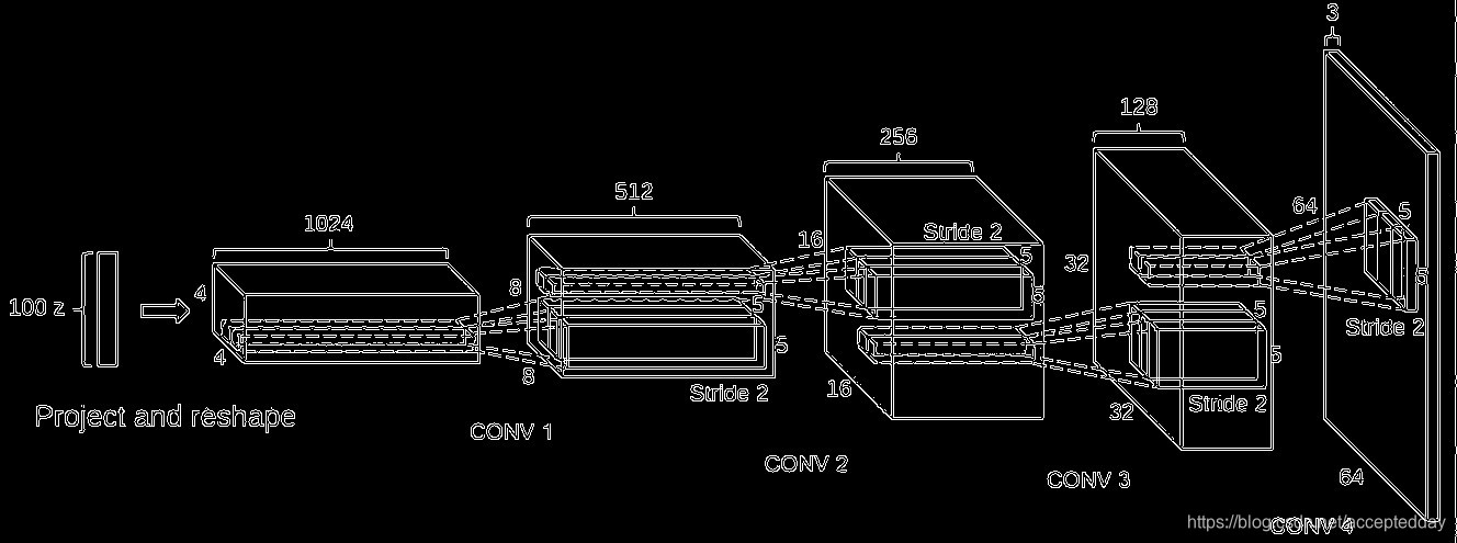
6.定义生成器(Generator)的网络结构:
def generator(z, is_training=is_training):
    momentum = 0.9
    with tf.variable_scope('generator', reuse=None):
        d = 4
        h0 = tf.layers.dense(z, units=d * d * 512)  # z是二维向量[None,[宽,高,通道数]],units是4*4*512个神经元
        h0 = tf.reshape(h0, shape=[-1, d, d, 512])
        h0 = tf.nn.relu(tf.contrib.layers.batch_norm(h0, is_training=is_training, decay=momentum))
        # 这里使用的是relu(),而不是lrelu()
        h1 = tf.layers.conv2d_transpose(h0, kernel_size=5, filters=256, strides=2, padding='same')
        h1 = tf.nn.relu(tf.contrib.layers.batch_norm(h1, is_training=is_training, decay=momentum))
        # shape[-1,8,8,256]

        h2 = tf.layers.conv2d_transpose(h1, kernel_size=5, filters=128, strides=2, padding='same')
        h2 = tf.nn.relu(tf.contrib.layers.batch_norm(h2, is_training=is_training, decay=momentum))
        # shape[-1,16,16,128]

        h3 = tf.layers.conv2d_transpose(h2, kernel_size=5, filters=64, strides=2, padding='same')
        h3 = tf.nn.relu(tf.contrib.layers.batch_norm(h3, is_training=is_training, decay=momentum))
        # shape[-1,32,32,64]

        h4 = tf.layers.conv2d_transpose(h3, kernel_size=5, filters=3, strides=2, padding='same', activation=tf.nn.tanh,
                                        name='g')
        # shape[-1,64,64,3]
        # 如果 padding='valid',则width+=(kernel_size-1),height+=(kernel_size-1)
        return h4
这里需要的注意是:
- 最终输出使用的是tanh()激活函数,观察sigmoid和tanh的函数曲线,sigmoid在输入处于[-1,1]之间时,函数值变化敏感 ,一旦接近或者超出区间就失去敏感性,处于饱和状态,影响神经网络预测的精度值。tanh的输出和输入能够保持非线性单调 上升和下降关系,容错性好,有界,渐进于0、1,符合人脑神经饱和的规律,但比sigmoid函数延迟了饱和期。
- 同时要注意image_shape的变换,生成器的思路是逆向复原输入的人脸图片。
7.得到fake的假人脸图片,经判别器映射之后的输入图片,未经sigmoid激活的输入图片的输出层数据,以及返回generator,discriminator中所有可训练的变量。
g = generator(noise)  # 生成噪音,烦扰项
d_real, d_real_logits = discriminator(X)
d_fake, d_fake_logits = discriminator(g, reuse=True)

vars_g = [var for var in tf.trainable_variables() if var.name.startswith('generator')]
vars_d = [var for var in tf.trainable_variables() if var.name.startswith('discriminator')]
# 返回generator,discriminator中所有可训练的变量
8.定义生成器和判别器的Loss函数。
loss_d_real = tf.reduce_mean(sigmoid_cross_entropy_with_logits(d_real_logits, tf.ones_like(d_real)))  # loss_d_real趋近于1,得分初始化为0~1
loss_d_fake = tf.reduce_mean(sigmoid_cross_entropy_with_logits(d_fake_logits, tf.zeros_like(d_fake)))  # loss_d_fake趋近于0
loss_g = tf.reduce_mean(sigmoid_cross_entropy_with_logits(d_fake_logits, tf.ones_like(d_fake)))  # loss_g 趋近于1
loss_d = loss_d_real + loss_d_fake
这里需要注意:
- Loss_d由loss_d_real和loss_d_fake组成。
- 我们希望loss_d_fake得分低,但是希望loss_g的得分高,因为d_fake得分越高,说明我们的假人脸图片越真实。(这是需要注意的细节。)
9.定义更新训练操作:
update_ops = tf.get_collection(tf.GraphKeys.UPDATE_OPS)
with tf.control_dependencies(update_ops):
    optimizer_d = tf.train.AdamOptimizer(learning_rate=0.0002, beta1=0.5).minimize(loss_d, var_list=vars_d)
    optimizer_g = tf.train.AdamOptimizer(learning_rate=0.0002, beta1=0.5).minimize(loss_g, var_list=vars_g)
10.定义读取图片函数:
def read_image(path, height, width):
    image = imread(path)
    h = image.shape[0]
    w = image.shape[1]

    if h > w:
        image = image[h // 2 - w // 2: h // 2 + w // 2, :, :]  # 将图片裁剪趋近于正方形。
    else:
        image = image[:, w // 2 - h // 2: w // 2 + h // 2, :]

    image = cv2.resize(image, (height, width))
    return image / 255.#归一化操作
需要注意的地方:
- 因为我们设定的宽高是64:64,所以对image[0,1,2]采取切片操作将图片裁剪趋近于64:64。
11.定义合并fake图片的函数:
def montage(images):
    if isinstance(images, list):
        images = np.array(images)
    img_h = images.shape[1]
    img_w = images.shape[2]
    n_plots = int(np.ceil(np.sqrt(images.shape[0])))
    if len(images.shape) == 4 and images.shape[3] == 3:
        m = np.ones(
            (images.shape[1] * n_plots + n_plots + 1,
             images.shape[2] * n_plots + n_plots + 1, 3)) * 0.5
    elif len(images.shape) == 4 and images.shape[3] == 1:
        m = np.ones(
            (images.shape[1] * n_plots + n_plots + 1,
             images.shape[2] * n_plots + n_plots + 1, 1)) * 0.5
    elif len(images.shape) == 3:
        m = np.ones(
            (images.shape[1] * n_plots + n_plots + 1,
             images.shape[2] * n_plots + n_plots + 1)) * 0.5
    else:
        raise ValueError('Could not parse image shape of {}'.format(images.shape))
    for i in range(n_plots):
        for j in range(n_plots):
            this_filter = i * n_plots + j
            if this_filter < images.shape[0]:
                this_img = images[this_filter]
                m[1 + i + i * img_h:1 + i + (i + 1) * img_h,
                1 + j + j * img_w:1 + j + (j + 1) * img_w] = this_img
    return m#这里只需知道经过合并处理之后的是一张10*10的100张fake人脸的合并图即可。
12.定义session(),fake的原始随机点,loss以及samples。
sess = tf.Session()
sess.run(tf.global_variables_initializer())
z_samples = np.random.uniform(-1.0, 1.0, [batch_size, z_dim]).astype(np.float32)  # 使用这里的随机值进行生成fake图片
samples = []  # 存放生成的fake图片
loss = {'d': [], 'g': []}  # 记录损失值
13.写for in in range( )大循环,进行迭代训练。
offset = 0
for i in range(60000):
    n = np.random.uniform(-1.0, 1.0, [batch_size, z_dim]).astype(np.float32)  # n:每次生成新的随机噪声

    offset = (offset + batch_size) % len(images)

    batch = np.array([read_image(img, HEIGHT, WIDTH) for img in images[offset: offset + batch_size]])# generator的tanh为(-1,1),而discriminator的sigmoid取值范围为(0,1),这里需要将batch的值映射到(-1,1)再进行训练。
    batch = (batch - 0.5) * 2

    d_ls, g_ls = sess.run([loss_d, loss_g], feed_dict={X: batch, noise: n, is_training: True})  # 每次使用新的随机噪声进行训练
    loss['d'].append(d_ls)
    loss['g'].append(g_ls)

    sess.run(optimizer_d, feed_dict={X: batch, noise: n, is_training: True})
    sess.run(optimizer_g, feed_dict={X: batch, noise: n, is_training: True})
    sess.run(optimizer_g, feed_dict={X: batch, noise: n, is_training: True})  # 每训练1次判别器,训练2次生成器
        if i % 500 == 0:
        	print(i, d_ls, g_ls)
        	gen_imgs = sess.run(g, feed_dict={noise: z_samples, is_training: False})  # z_samples在训练过程中是不变的
        	gen_imgs = (gen_imgs + 1) / 2
        	imgs = [img[:, :, :] for img in gen_imgs]
        	gen_imgs = montage(imgs)
        	imsave(os.path.join(OUTPUT_DIR, 'sample_%d.jpg' % i), gen_imgs)
        	samples.append(gen_imgs)
相关的注意点:
- n:每次生成新的随机噪声,每次使用新的随机噪声进行训练。z_samples:原始随机噪声,用于生成人脸图片,在训练过程中是不变的。
- 由于判别器通常比生成器收敛的快,所以每训练1次判别器,训练2次生成器。
- 每训练500次,打印loss_d和loss_g的值,同时使用z_samples生成fake人脸图片并保存。
14.保存模型
saver = tf.train.Saver()
saver.save(sess, os.path.join(OUTPUT_DIR, 'dcgan_' + dataset), global_step=60000)
15.训练过程的GIF动态展示