常见统计分布的概率分布图

import numpy as np
import matplotlib.pyplot as plt
import seaborn as sns
from scipy import stats
sns.set()
sns.set_style('ticks')
sns.set_context('talk')
%matplotlib inline

Normal distribution

x = np.linspace(-5, 5, 40)
plt.figure(figsize=(14, 5))

# probability density function
plt.subplot(121)
for sigma in (0.4, 1, 1.4):
    plt.plot(x, stats.norm.pdf(x, loc=0, scale=sigma), label=f'$\sigma={sigma}$')
plt.legend()
sns.despine()
plt.title('pdf of normal distribution') #fontdict={'fontsize':16}

# cumulative distribution function
plt.subplot(122)
for sigma in (0.4, 1, 1.4):
    plt.plot(x, stats.norm.cdf(x, loc=0, scale=sigma), label=f'$\sigma={sigma}$')
plt.legend()
sns.despine()
plt.title('cdf of normal distribution') #fontdict={'fontsize':16})
plt.show()

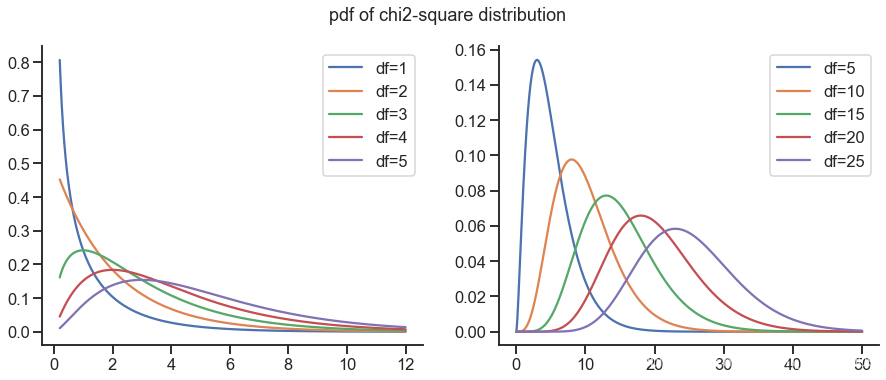
$\chi^2$ distribution

$f(x, k) = \displaystyle\frac{1}{2^{k/2} \Gamma \left( k/2 \right)}x^{k/2-1} \exp \left( -x/2 \right)$

plt.figure(figsize=(15, 5.5))

plt.subplot(121)
x = np.linspace(0.2, 12, 2000)
for k in range(1, 6, 1):
    plt.plot(x, stats.chi2.pdf(x, df=k), label=f'df={k}')
plt.legend()
sns.despine()

plt.subplot(122)
x = np.linspace(0, 50, 2000)
for k in range(5, 30, 5):
    plt.plot(x, stats.chi2.pdf(x, df=k), label=f'df={k}')
plt.legend()
sns.despine()
plt.suptitle('pdf of chi2-square distribution', fontsize=18)
plt.show()

plt.figure(figsize=(15, 5.5))

plt.subplot(121)
x = np.linspace(0.2, 12, 2000)
for k in range(1, 6, 1):
    plt.plot(x, stats.chi2.cdf(x, df=k), label=f'df={k}')
plt.legend()
sns.despine()

plt.subplot(122)
x = np.linspace(0, 50, 2000)
for k in range(5, 30, 5):
    plt.plot(x, stats.chi2.cdf(x, df=k), label=f'df={k}')
plt.legend()
sns.despine()
plt.suptitle('cdf of chi2-square distribution', fontsize=18)
plt.show()

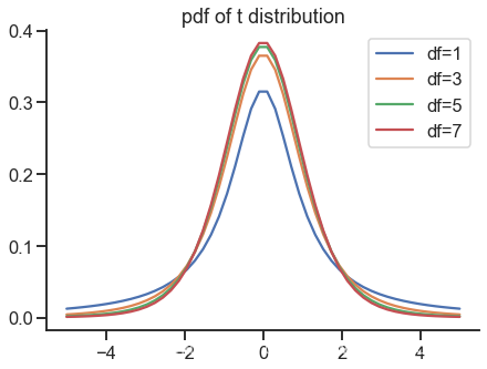
t-distribution

$f(x, \nu) = \displaystyle\frac{\Gamma((\nu+1)/2)} {\sqrt{\pi \nu} \Gamma(\nu)} (1+x^2/\nu)^{-(\nu+1)/2}$

plt.figure(figsize=(7, 5))
x = np.linspace(-5, 5)
for k in range(1, 8, 2):
    plt.plot(x, stats.t.pdf(x, df=k), label=f'df={k}')
plt.legend()
sns.despine()
plt.title('pdf of t distribution')
plt.show()

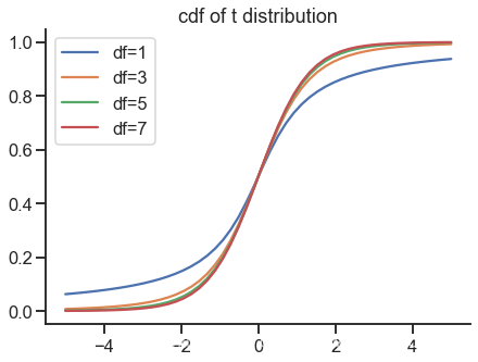
plt.figure(figsize=(7, 5))
x = np.linspace(-5, 5)
for k in range(1, 8, 2):
    plt.plot(x, stats.t.cdf(x, df=k), label=f'df={k}')
plt.legend()
sns.despine()
plt.title('cdf of t distribution')
plt.show()

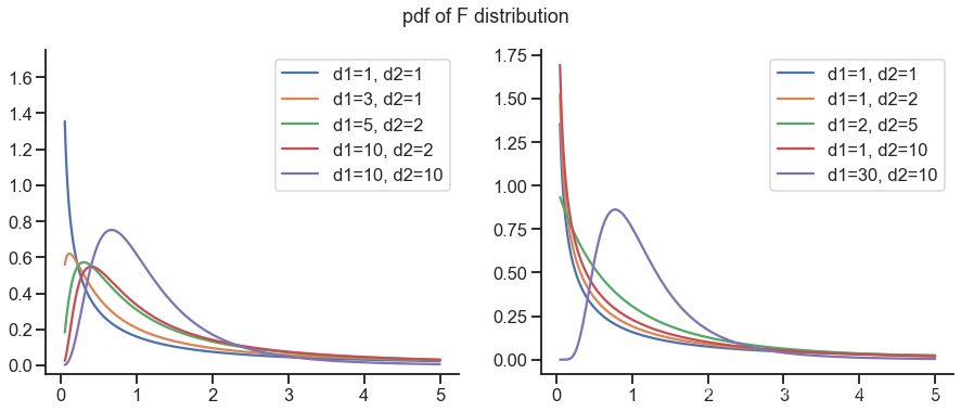
F-distribution

x = np.linspace(0.05, 5, 400)
plt.figure(figsize=(15, 5.5))

plt.subplot(121)
for d1, d2 in [(1, 1), (3, 1), (5, 2), (10, 2), (10, 10)]:
    y = stats.f.pdf(x, d1, d2)
    plt.ylim(-0.05, 1.75)
    plt.plot(x, y, label=f'd1={d1}, d2={d2}')
plt.legend()
sns.despine()

plt.subplot(122)
for d1, d2 in [(1, 1), (1, 2), (2, 5), (1, 10), (30, 10)]:
    y = stats.f.pdf(x, d1, d2)
    plt.plot(x, y, label=f'd1={d1}, d2={d2}')
plt.legend()
sns.despine()

plt.suptitle('pdf of F distribution', fontsize=18)
plt.show()

x = np.linspace(0.05, 5, 400)
plt.figure(figsize=(15, 5.5))

plt.subplot(121)
for d1, d2 in [(1, 1), (3, 1), (5, 2), (10, 2), (10, 10)]:
    y = stats.f.cdf(x, d1, d2)
    plt.plot(x, y, label=f'd1={d1}, d2={d2}')
plt.legend()
sns.despine()

plt.subplot(122)
for d1, d2 in [(1, 1), (1, 2), (2, 5), (1, 10), (30, 10)]:
    y = stats.f.cdf(x, d1, d2)
    plt.plot(x, y, label=f'd1={d1}, d2={d2}')
plt.legend()
sns.despine()

plt.suptitle('cdf of F distribution', fontsize=18)
plt.show()

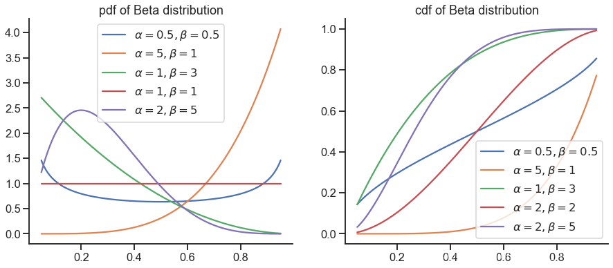
Beta distribution

x = np.linspace(0.05, 0.95, 400)
plt.figure(figsize=(15, 6))

plt.subplot(121)
for alpha, beta in [(0.5, 0.5), (5, 1), (1, 3), (1, 1), (2, 5)]:
    plt.plot(x, stats.beta.pdf(x, alpha, beta), label=r'$\alpha={}, \beta={}$'.format(alpha, beta))
plt.legend()
sns.despine()
plt.title('pdf of Beta distribution')

plt.subplot(122)
for alpha, beta in [(0.5, 0.5), (5, 1), (1, 3), (2, 2), (2, 5)]:
    plt.plot(x, stats.beta.cdf(x, alpha, beta), label=r'$\alpha={}, \beta={}$'.format(alpha, beta))
plt.legend()
sns.despine()
plt.title('cdf of Beta distribution')
plt.show()

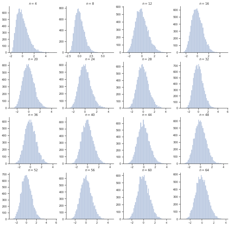
对中心极限定理的验证

$\epsilon_n=\displaystyle\frac{S_n-n\mu}{\sqrt{n\sigma^2}} \rightarrow_d \mathcal{N}(0, 1)$。
目标是考察 $\epsilon_2, \epsilon_3, \epsilon_4,\cdots, \epsilon_{100}, \epsilon_...$ 的分布情况
以参数为 1 的指数分布为例

sns.set_context('notebook')

plt.figure(figsize=(15, 15))
for i in range(1, 17):
    plt.subplot(4, 4, i)
    n = 4 * i
    rvs = [
        (np.random.exponential(size=n).sum() - n) / np.sqrt(n)
        for _ in range(10000)
        ]
    sns.distplot(rvs, kde=False)
    plt.title(f"$n={n}$");sns.despine()
plt.show()

参数为 1 的泊松分布，这是一个离散型的分布

plt.figure(figsize=(15, 15))
for i in range(1, 17):
    plt.subplot(4, 4, i)
    n = 20 * i
    rvs = [
        (np.random.poisson(size=n).sum() - n) / np.sqrt(n)
        for _ in range(5000)
        ]
    sns.distplot(rvs, kde=False)
    plt.title(f"$n={n}$");sns.despine()
plt.show()

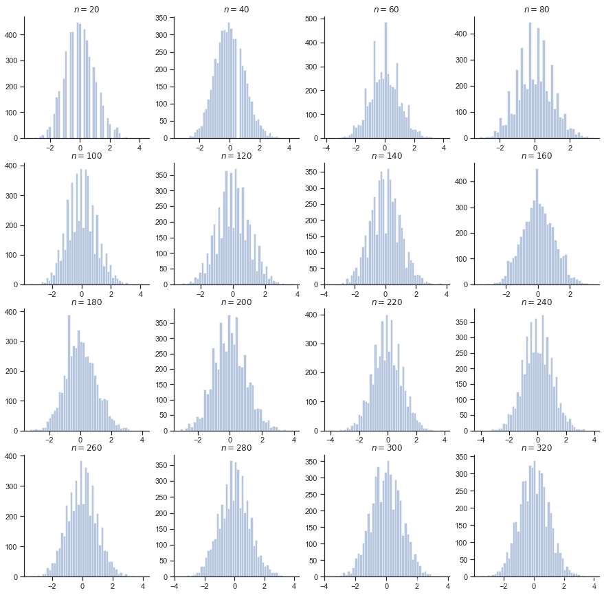
从上面可以看到，对于一个连续型的分布，它的“标准型”能够更快的趋近于正态分布。而对于离散型分布而言，它所需要的 $n$ 可能就比较大了。