Regularization - Regularized linear regression

摘要: 本文是吴恩达 (Andrew Ng)老师《机器学习》课程，第八章《正则化》中第57课时《正则化线性回归》的视频原文字幕。为本人在视频学习过程中记录下来并加以修正，使其更加简洁，方便阅读，以便日后查阅使用。现分享给大家。如有错误，欢迎大家批评指正，在此表示诚挚地感谢！同时希望对大家的学习能有所帮助。

For linear regression, we have previously worked out two learning algorithms, one based on gradient descent, and one based on the normal equation. In this video we will take those two algorithms and generalize them to the case of regularized linear regression.

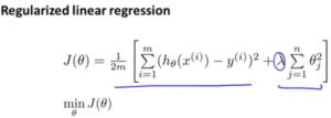
Here’s the optimization objective that we came up last time for regularized linear regression. This first part is our usual objective for linear regression, and now we have this additional regularization term, where $\lambda$ is our regularization parameter. And we like to find parameters $\theta$ that minimizes this cost function, this regularized cost function $J(\theta )$ .

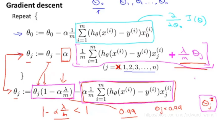
Previously, we were using gradient descent for the original cost function without the regularization term, and we had the following algorithm for regular linear regression without regularization. We’ll repeatedly update the parameters $\theta _{j}$ as follows, for j=1,2…n. Let me take this and just write the case for $\theta _{0}$ separately. So, I’m just gonna write the update for Θ0 separately, then for the update, for the parameters, 1, 2, 3 and so on up to n. So, I haven’t changed anything yet, right? This is just writing the update for $\theta _{0}$ separately from the updates from $\theta _{1}$ , $\theta _{2}$ , $\theta _{3}$ , up to $\theta _{n}$ . And the reason I want to do this is, you may remember that for our regularized linear regression, we penalized the parameters $\theta _{1}$ , $\theta _{2}$ , $\theta _{3}$ , up to $\theta _{n}$ , But we don’t penalize $\theta _{0}$ . So when we modify this algorithm for regularized linear regression, we’re going to end up treating $\theta _{0}$ slightly differently. Concretely, if we want to take this algorithm and modify it to use the regularized objective, all we need to do is take this term at the bottom and modify as follows. We’re gonna take this term and add $-\frac{\lambda }{m}\theta _{j}$ . And if you implement this, then you have gradient descent for trying to minimize the regularized cost function $J(\theta )$ . And concretely, I’m not gonna do the calculus to prove it, But concretely if you look at this term, this term that’s written in this square brackets, if you know calculus, it’s possible to prove that that term is the partial derivative, with respect to $J(\theta )$ , using the new definition of $J(\theta )$ with the regularization term. And similarly on this term up on top, which I guess I am drawing the salient box, that’s still the partial derivative respect to $\theta _{0}$ for $J(\theta )$ . If you look at the update for $\theta _{j}$ , it’s possible to show something pretty interesting. Concretely, $\theta _{j}$ gets updated as $\theta _{j}$ minus $\alpha$ times, and then you have this other term here that depends on $\theta _{j}$ . So if you group all the terms together that depending on $\theta _{j}$ , you can show that this update can be written equivalently as follows, and all I did was have $\theta _{j}$ , here is $\theta _{j}$ times 1, and this term is $\frac{\lambda }{m}$ , so you end up with $\alpha \frac{\lambda }{m}$ , multiply them to $\theta _{j}$ . And this term here, $1-\alpha \frac{\lambda }{m}$ here, is a pretty interesting term, and it has a pretty interesting effect. Concretely, this term, $1-\alpha \frac{\lambda }{m}$ is going to be a number that’s usually a number that’s a little bit less than 1 because $\alpha \frac{\lambda }{m}$ is going to be positive, and usually, if your learning rate is small and m is large, that’s usually pretty small. So this term here, it’s going to be a number, it’s usually, a little bit less than 1. So think of it as a number like 0.99, let’s say. And so the effect of our updates of $\theta _{j}$ is, we’re going to say that $\theta _{j}$ gets replaced by $\theta _{j}$ times 0.99. So $\theta _{j}$ times 0.99 has the effect of shrinking $\theta _{j}$ a little bit towards 0. So this makes $\theta _{j}$ a bit smaller. More formally, this makes this square norm of $\theta _{j}$ ( $\theta _{j}^{2}$ )a little bit smaller. And then after that, the 2nd term here, that’s actually exactly the same as the original gradient descent updated that we had before we added all this regularization stuff. So, hopefully this gradient descent, hopefully this update makes sense. When we’re using regularized linear regression what we’re doing is on every iteration, we’re multiplying $\theta _{j}$ by a number that’s a little bit less than 1. So we’re shrinking the parameter a little bit, and then we’re performing similar update as before. Of course that’s just the intuition behind what this particular update is doing. Mathematically, what it’s doing is exactly gradient descent on the cost function $J(\theta )$ , that we defined on the previous slide that uses the regularization term.

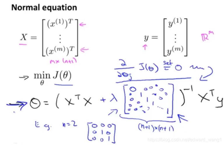
Gradient descent was just one of our two algorithms for fitting a linear regression model. The 2nd algorithm was the one based on the normal equation, where, what we did was we created the design matrix “X”, where each row corresponded to a separate training example. And we created a vector y, so this is a vector that is an m dimensional vector, and that contain the labels from a training set. So whereas X is an m x (n+1) matrix. y is an m dimensional vector. And in order to minimize the cost function $J(\theta )$ , we found that one way to do so is to set $\theta$ to equal to this: $\theta =(X^{T}X)^{-1}X^{T}y$ . I’m leaving room here, to fill in stuff of course. And what this value for $\theta$ does is minimizes the cost function $J(\theta )$ , when we were not using regularization. Now that we’re using regularization, if you were to derive what the minimum is, and just give you a sense of how to derive the minimum. The way you derive it is you take partial derivatives in respect to each parameter, set this 0, and then do a bunch of math, and you can then show that, it’s a formula like this, that minimizes the cost function. And concretely, if you’re using regularization, then this formula changes as follows. Inside this parenthesis, you end up with a matrix like this: 0 1 1 and so on, 1 until the bottom. So this thing over here is a matrix, whose upper leftmost entry is 0, there’s ones on the diagonals, and then the zeros everywhere else on this matrix. Because I’m drawing this a little bit sloppy. But as a concrete example, if n=2, then this matrix is going to be a 3×3 matrix. More generally, this matrix is a (n+1) x (n+1) dimensional matrix. So n=2, then that matrix becomes something that looks like this. And once again, I’m not going to show those derivation which is frankly somewhat long and involved. But it is possible to prove that if you are using the new definition of $J(\theta )$ with the regularization objective, then this new formula for $\theta$ is the one that will give you the global minimum of $J(\theta )$ .

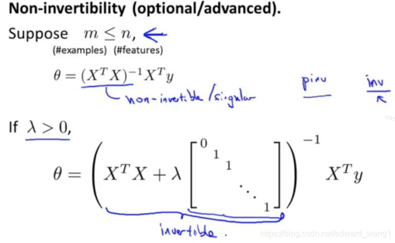
So finally, I want to just quickly describe the issue of non-invertibility. This is relatively advanced material. So you should consider this as optional and feel free to skip it, or if you listen to it and possibly it don’t really make sense, don’t worry about it either. But earlier when I talked about the normal equation method, we also had an optional video on the non-invertibility issue. So this is another optional part, that is sort of add on to that earlier optional video on non-invertibility. Now considering setting where m, the number of example is less than or equal to n, the number of features. If you have fewer examples than features, then this matrix $X^{T}X$ will be non-invertible, or singular, or the other term for this is the matrix will be degenerate. And if you implement this in Octave, anyway and you use the pinv function to take the pseudo inverse kind to do the right thing, but it’s not clear that it will give you a very good hypothesis. Even though numerically the Octave pinv function will give you a result that kind of make sense. But if you were doing this in a different language, and if you were taking just the regular inverse, which in Octave is denoted with the function inv, we’re trying to take the regular inverse of $X^{T}X$ , then in this setting, you find that $X^{T}X$ is singular, is non-invertible, and if you’re doing this in a different programming language, and using some linear algebra library, to try to take the inverse of this matrix, it just might not work, because that matrix is non-invertible or singular. Fortunately, regularization also takes care of this for us. And concretely, so long as the regularization parameter λ is strictly greater than 0, it’s actually possible to prove that this matrix $X^{T}X$ plus λ times this funny matrix here, it is possible to prove that this matrix will not be singular, and that this matrix will be invertible. So using regularization also takes care of any non-invertibility issues of the $X^{T}X$ matrix as well.

So you now know how to implement regularized linear regression. Using this, you’ll be able to avoid overfitting, even if you have lots of features in a relatively small training set. And this should let you get linear regression to work much better for many problems. In the next video, we’ll take this regularization idea and apply it to logistic regression. So that you’ll be able to get logistic regression to avoid overfitting, and perform much better as well.

<end>

王彩旗

发布了41 篇原创文章 · 获赞 12 · 访问量 1306

私信关注

Regularization - Regularized linear regression

猜你喜欢