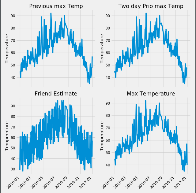
第一步: 进行特征的可视化操作
import pandas as pd
import numpy as np
import datetime
import matplotlib.pyplot as plt

features = pd.read_csv('temps.csv')

# 可视化图形
print(features.head(5))

#使用日期构造可视化图像
dates = [str(int(year)) + "-" + str(int(month)) + "-" + str(int(day)) for year, month, day in zip(features['year'], features['month'], features['day'])]
dates = [datetime.datetime.strptime(date, "%Y-%m-%d") for date in dates]

# 进行画图操作
plt.style.use("fivethirtyeight")

fig, ((ax1, ax2), (ax3, ax4)) = plt.subplots(nrows=2, ncols=2, figsize=(10, 10))
fig.autofmt_xdate(rotation=45)

ax1.plot(dates, features["temp_1"])
ax1.set_xlabel('')
ax1.set_ylabel('Temperature')
ax1.set_title("Previous max Temp")

ax2.plot(dates, features["temp_2"])
ax2.set_xlabel('')
ax2.set_ylabel('Temperature')
ax2.set_title("Two day Prio max Temp")

ax3.plot(dates, features["friend"])
ax3.set_xlabel('')
ax3.set_ylabel('Temperature')
ax3.set_title("Friend Estimate")

ax4.plot(dates, features["actual"])
ax4.set_xlabel('')
ax4.set_ylabel('Temperature')
ax4.set_title("Max Temperature")

plt.tight_layout(pad=2)
plt.show()
第二步: 对非数字的特征进行独热编码,使用温度的真实值作为标签,去除真实值的特征作为输入特征,同时使用process进行标准化操作
# 构造独热编码
# 遍历特征,将里面不是数字的特征进行去除
for feature_name in features.columns:
    print(feature_name)
    try:
        float(features.loc[0, feature_name])
    except:
        for s in set(features[feature_name]):
            features[s] = 0

        #根据每一行数据在时间特征上添加为1
        for f in range(len(features)):
            features.loc[f, [features.iloc[f][feature_name]]] = 1

        # 去除对应的week特征
        features = features.drop(feature_name, axis=1)

# 构造独热编码也可以使用
# features = pd.get_dummies(features)

# 构造标签
labels = np.array(features['actual'])

# 构造特征
features = features.drop('actual', axis=1)

# 进行torch网络训练
import torch

# 对特征进行标准化操作
from sklearn import preprocessing

input_feature = preprocessing.StandardScaler().fit_transform(features)


print(input_feature[:, 5])
第三步: 对特征和标签进行torch.tensor处理,转换为tensor格式,初始化weigh和biases, 使用batch_size进行迭代优化,利用weight.grad 和 biases.grad进行学习率的梯度优化
# 构建神经网络
x = torch.tensor(input_feature, dtype=torch.float)

y = torch.tensor(labels, dtype=torch.float)


weight = torch.randn((14, 128), dtype=torch.float, requires_grad=True)
biases = torch.randn(128, dtype=torch.float, requires_grad=True)

weight2 = torch.randn((128, 1), dtype=torch.float, requires_grad=True)
biases2 = torch.randn(1, dtype=torch.float, requires_grad=True)

learning_rate = 0.001
losses = []
batch_size = 16


for i in range(1000):
    # 计算隐层
    batch_loss = []
    for start in range(0, len(input_feature), batch_size):
        end = start + batch_size if start + batch_size < len(input_feature) else len(input_feature)
        xx = torch.tensor(input_feature[start:end], dtype=torch.float, requires_grad=True)
        yy = torch.tensor(labels[start:end], dtype=torch.float, requires_grad=True)
        hidden = xx.mm(weight) + biases
        # 加入激活函数
        hidden = torch.sigmoid(hidden)
        #预测结果
        predictions = hidden.mm(weight2) + biases2
        # 计算损失值
        loss = torch.mean((predictions - yy) ** 2)
        loss.backward()

        # 更新参数
        weight.data.add_(- learning_rate * weight.grad.data)
        biases.data.add_(- learning_rate * biases.grad.data)
        weight2.data.add_(- learning_rate * weight2.grad.data)
        biases2.data.add_(- learning_rate * biases2.grad.data)

        # 每次迭代都记得清空
        weight.grad.data.zero_()
        biases.grad.data.zero_()
        weight2.grad.data.zero_()
        biases2.grad.data.zero_()
        batch_loss.append(loss.data.numpy())
    if i % 100 == 0:
        losses.append(np.mean(batch_loss))
        print(i, np.mean(batch_loss))
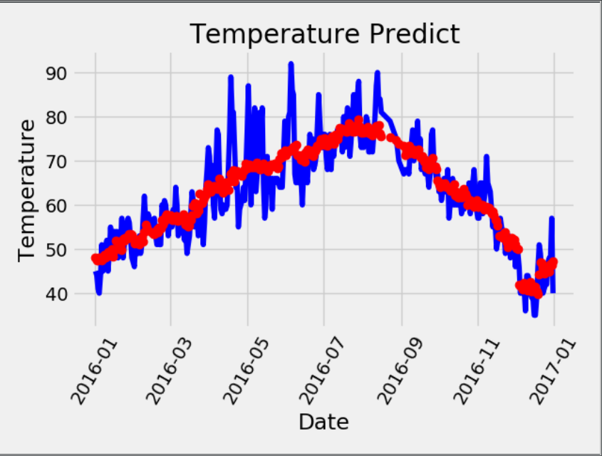
第四步: 将x重新输入到网络中,计算获得最终的prediction,进行最终的作图
hidden = x.mm(weight) + biases
# 加入激活函数
hidden = torch.sigmoid(hidden)
# 预测结果
prediction = hidden.mm(weight2) + biases2

prediction = prediction.detach().numpy()
plt.plot(dates, y, 'b-', label='actual')
plt.plot(dates, prediction, 'ro', label='predit')
plt.xticks(rotation=60)
plt.title("Temperature Predict")
plt.xlabel("Date")
plt.ylabel("Temperature")
plt.show()