一篇文章搞懂Numpy的Python学习指北(文末附应用举例)

大家在刚开始学python时,有没有pip install numpy呢?下面我们一起来学习一下:

Numpy是NumericalPython的简称，是Python中高性能科学计算和数据分析的基础包。ndarray数组是Numpy中的基础数据结构式，它具有矢量算术运算和复杂广播的能力，可以实现快速的计算并且能节省存储空间。

在Python中使用list列表可以非常灵活的处理多个元素的操作，但是其效率却比较低。ndarray数组相比于Python中的list列表更加方便,下面我们做一下对比学习:

ndarray数组中所有元素的数据类型是相同的，数据地址是连续的，批量操作数组元素时速度更快；list列表中元素的数据类型可以不同，需要通过寻址方式找到下一个元素
ndarray数组中实现了比较成熟的广播机制，矩阵运算时不需要写for循环
Numpy底层是用c语言编写的，内置了并行计算功能，运行速度高于纯Python代码

下面一起来看看使用list列表和ndarray数组完成相同的任务，两种方式在代码上的区别,下面说一下我的代码结构:

import numpy as np

def method_1():  #list列表
    a1 = [1, 2, 3, 4, 5]
    b1 = [1, 2, 3, 4, 5]

def method_2():  #ndarray数组
    a2 = np.array([1, 2, 3, 4, 5])
    b2 = np.array([1, 2, 3, 4, 5])

def main():
    method_1()
    method_2()

if __name__ == '__main__':
    main()

方法1里使用list列表,变量a1、b1表示方法1里的列表;
方法2里使用ndarray数组,变量a2、b2表示方法2里的数组。

下面的代码中只展示method_1与method_2里的代码,而main函数内容不变,故省略

ndarray数组和list列表分别完成对每个元素同时进行加减乘除的计算

def method_1():
    a1 = [1, 2, 3, 4, 5]
    b1 = [1, 2, 3, 4, 5]
    for i in range(5):
        a1[i] = a1[i] + 1
        b1[i] = b1[i] * 2
    print("a1:",a1)
    print("b1:",b1)

在这里插入图片描述

def method_2():
    a2 = np.array([1, 2, 3, 4, 5])
    b2 = np.array([1, 2, 3, 4, 5])
    a2 = a2 + 1
    b2 = b2 * 2
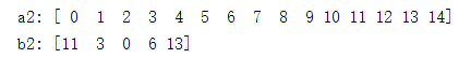
    print("a2:",a2)
    print("b2:",b2)

在这里插入图片描述

ndarray数组和list列表对应元素分别完成相加计算

在列表里,我们直接相加:
在这里插入图片描述
这样的效果不是我们想要的,看来,我们还是要用循环:

def method_1():
    a1 = [1, 2, 3, 4, 5]
    b1 = [1, 2, 3, 4, 5]
    c1 = []
    for i in range(5):
        c1.append(a1[i] + b1[i])
    print("c1:",c1)

在这里插入图片描述

def method_2():
    a2 = np.array([1, 2, 3, 4, 5])
    b2 = np.array([1, 2, 3, 4, 5])
    c2 = a2 + b2
    print("c2:",c2)

在这里插入图片描述
从上面的示例中可以看出，使用ndarray数组不需要写for循环，就可以非常方便的完成数学计算，在操作矢量或者矩阵时，可以像操作普通的数值变量一样编写程序，使得代码极其简洁。

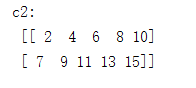
另外，ndarray数组还提供了广播机制，它会按一定规则自动对数组的维度进行扩展以完成计算，如下面例子所示，1维数组和2维数组进行相加操作，ndarray数组会自动扩展1维数组的维度，然后再对每个位置的元素分别相加:

def method_2():
    # 二维数组维度 2x5
    a2 = np.array([[1, 2, 3, 4, 5],
                   [6, 7, 8, 9, 10]])
    # 一维数组维度 1x5
    b2 = np.array([1, 2, 3, 4, 5])
    c2 = a2 + b2
    print("c2:\n",c2)

在这里插入图片描述
既然使用数组可以提高我们的体验感,那么下面我们就来看看它的创建方法

ndarray数组的创建方法

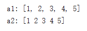
我们可以把列表转换成数组:

def method_1():
    a1 = [1, 2, 3, 4, 5]
    print("a1:",a1)
    a2 = np.array(a1)
    print("a2:",a2)

在这里插入图片描述
使用np.arange,通过指定start, stop , interval来产生一个1维的ndarray:

def method_2():
    a2 = np.arange(0, 20, 2)
    print("a2:",a2)

在这里插入图片描述
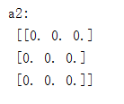
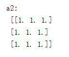
我们还可以创建一个全零的或者是全1的数组:

def method_2():
    a2 = np.zeros([3,3])
    print("a2:\n",a2)

在这里插入图片描述

def method_2():
    a2 = np.ones([3,3])
    print("a2:\n",a2)

在这里插入图片描述

数组有属于自己的属性,下面一起来看看查询它的方法

查看ndarray数组的属性

ndarray的属性包括形状shape、数据类型dtype、元素个数size和维度ndim等:

数组的数据类型 ndarray.dtype
数组的形状 ndarray.shape，1维数组(N, )，二维数组(M, N)，三维数组(M, N, K)
数组的维度大小，ndarray.ndim, 其大小等于ndarray.shape所包含元素的个数
数组中包含的元素个数 ndarray.size，其大小等于各个维度的长度的乘积

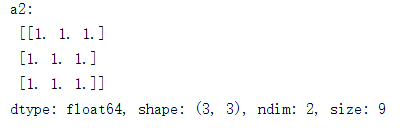
def method_2():
    a2 = np.ones([3,3])
    print("a2:\n",a2)
    print('dtype: {}, shape: {}, ndim: {}, size: {}'.format(a2.dtype, a2.shape, a2.ndim, a2.size))

在这里插入图片描述
创建ndarray之后，可以对其数据类型进行更改，或者对形状进行调整

改变ndarray数组的数据类型和形状

def method_2():
    a2 = np.ones([3,3])
    print("a2:\n",a2)
    print('dtype: {}, shape: {}, ndim: {}, size: {}'.format(a2.dtype, a2.shape, a2.ndim, a2.size))
    # 转化数据类型
    b2 = a2.astype(np.int64)
    print("b2:\n",b2)
    print('b2, dtype: {}, shape: {}'.format(b2.dtype, b2.shape))
    # 改变形状
    c2 = a2.reshape([1, 9])
    print("c2:\n",c2)
    print('c2, dtype: {}, shape: {}'.format(c2.dtype, c2.shape))

在这里插入图片描述
ndarray数组的基本运算

ndarray数组可以像普通的数值型变量一样进行加减乘除操作

标量和ndarray数组之间的运算在开头已经讲过了,这里就不过多去阐述了,下面来看看两个ndarray数组之间的运算

def method_2():
    a2 = np.ones([2,5])
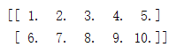
    b2 = np.array([[1, 2, 3, 4, 5],
                   [6, 7, 8, 9, 10]])

两个数组对应位置的元素相减:

	c2 = b2 -a2
    print(c2)

在这里插入图片描述
两个数组对应位置的元素相乘:

	c2 = b2 * a2
    print(c2)

在这里插入图片描述
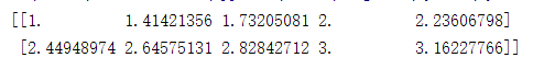
数组开根号，将每个位置的元素都开根号:

	c2 = b2 ** 0.5
    print(c2)

在这里插入图片描述
在程序中，通常需要访问或者修改ndarray数组某个位置的元素，也就是要用到ndarray数组的索引；有些情况下可能需要访问或者修改一些区域的元素，则需要使用数组的切片。

ndarray数组的索引和切片

索引和切片的使用方式与Python中的list类似，ndarray数组可以基于 -n ~ n-1 的下标进行索引，切片对象可以通过内置的 slice 函数，并设置 start, stop 及 step 参数进行，从原数组中切割出一个新数组。

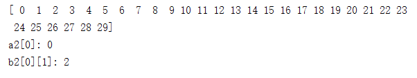
def method_2():
    a2 = np.arange(30)
    b2 = np.array([[1, 2, 3, 4, 5],
                   [6, 7, 8, 9, 10]])
    print(a2)
    print("a2[0]:",a2[0])
    print("b2[0][1]:",b2[0][1])

在这里插入图片描述

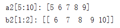
	print("a2[5:10]:",a2[5:10])
    print("b2[1:2]:",b2[1:2])

在这里插入图片描述
将一个标量值赋值给一个切片时，该值会自动传播到整个选区:

def method_2():
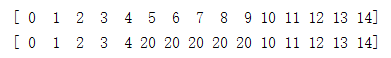
    a2 = np.arange(15)
    print(a2)
    a2[5:10] = 20
    print(a2)

在这里插入图片描述
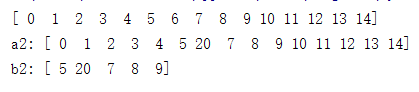
除此之外,视图上的任何修改都会直接反映到源数组上:

def method_2():
    a2 = np.arange(15)
    print(a2)
    b2 = a2[5:10]
    b2[1] = 20
    print("a2:",a2)
    print("b2:",b2)

在这里插入图片描述
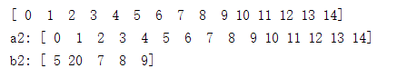
要想避免这种情况,我们可以通过copy()给新数组创建不同的内存空间:

def method_2():
    a2 = np.arange(15)
    print(a2)
    b2 = a2[5:10]
    b2 = np.copy(b2)
    b2[1] = 20
    print("a2:",a2)
    print("b2:",b2)

在这里插入图片描述
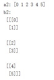
多维数组的索引和切片:

def method_2():
    a2 = np.arange(6)
    b2 = a2.reshape(3, 2, 1)
    print("a2:",a2)
    print("b2:\n",b2)

在这里插入图片描述
只有一个索引指标时，会在第0维上索引，后面的维度保持不变:

print("b2[0]:\n",b2[0])

在这里插入图片描述
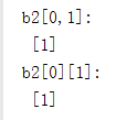
两个索引指标:

	print("b2[0,1]:\n",b2[0,1])
    print("b2[0][1]:\n",b2[0][1])

在这里插入图片描述
我们还可以使用python中的for语法对数组切片:

def method_2():
    a2 = np.arange(24)
    a2 = a2.reshape([6, 4])
    b2 = [a2[k:k+2] for k in range(0, 6, 2)] 
    print("a2:",a2)
    print("b2:\n",b2)

k in range(0, 6, 2) 决定了k的取值可以是0, 2, 4:
在这里插入图片描述

ndarray数组的统计运算

计算均值，使用arr.mean() 或 np.mean(arr)，二者是等价的:

def method_2():
    a2 = np.array([[1,2,3], [4,5,6], [7,8,9]])
    print("a2:",a2.mean())
    print("a2:",np.mean(a2))

在这里插入图片描述
除此之外还有:

求和 arr.sum(), np.sum(arr)
最大值 arr.max(), np.max(arr)
求最小值 arr.min(), np.min(arr)
找出最大元素的索引 arr.argmax(), arr.argmax(axis=0), arr.argmax(axis=1)
找出最小元素的索引 arr.argmin(), arr.argmin(axis=0), arr.argmin(axis=1)
计算标准差 arr.std()
计算方差 arr.var()

这里面可以指定参数:

def method_2():
    a2 = np.array([[1,2,3], [4,5,6], [7,8,9]])
    print("a2:",a2.mean(axis = 1))
    print("a2:",a2.sum(axis=0))

在这里插入图片描述
沿着第1维求平均，也就是将[1, 2, 3]取平均等于2，[4, 5, 6]取平均等于5，[7, 8, 9]取平均等于8;
沿着第0维求和，也就是将[1, 4, 7]求和等于12，[2, 5, 8]求和等于15，[3, 6, 9]求和等于18。

设置随机数种子

如果设置随机数种子，那么产生的随机数就不会变即每次运行结果一致:

def method_2():
    for i in range(3):
        np.random.seed(20)
        a2 = np.random.rand(3, 3)
        print("a2:",a2)

在这里插入图片描述
下面是不设置随机数种子生成的随机数:

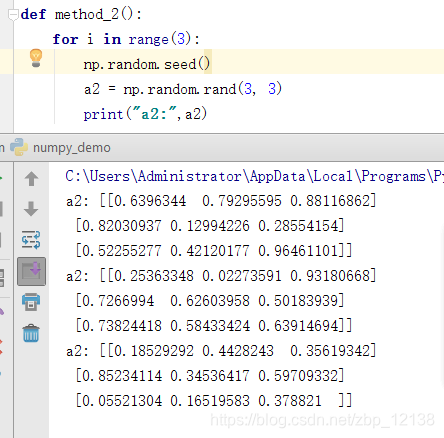
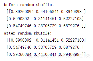
随机打乱ndarray数组顺序

def method_2():
    a2 = np.random.rand(3, 3)
    print('before random shuffle: \n', a2)
    np.random.shuffle(a2)
    print('after random shuffle: \n', a2)

在这里插入图片描述
这是1维数组,下面看看2维数组的:

def method_2():
    a2 = np.arange(0, 30)
    a2 = a2.reshape(6, 5)
    print('before random shuffle: \n', a2)
    np.random.shuffle(a2)
    print('after random shuffle: \n', a2)

在这里插入图片描述
随机打乱1维数组顺序时，发现所有元素位置都改变了；随机打乱二维数组顺序时，发现只有第行的顺序被打乱了，列的顺序保持不变。

随机选取元素

def method_2():
    a2 = np.arange(0, 15)
    b2 = np.random.choice(a2, size=5)
    print("a2:",a2)
    print("b2:",b2)

在这里插入图片描述
Numpy中实现了线性代数中常用的各种操作，并形成了numpy.linalg线性代数相关的模块:

线性代数

矩阵相乘:

def method_2():
    a2 = np.arange(12)
    b2 = a2.reshape([3, 4])
    c2 = a2.reshape([4, 3])
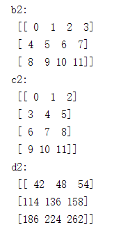
    print("b2:\n",b2)
    print("c2:\n",c2)
    # 矩阵b的第二维大小，必须等于矩阵c的第一维大小
    d2 = b2.dot(c2) # 等价于 np.dot(b, c)
    print("d2:\n",d2)

在这里插入图片描述
学过线性代数应该知道,矩阵b与c相乘时矩阵b的第二维大小，必须等于矩阵c的第一维大小

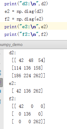
	e2 = np.diag(d2)
    f2 = np.diag(e2)
    print("e2:\n",e2)
    print("f2:\n",f2)

使用diag 可以用一维数组的形式返回方阵的对角线（或非对角线）元素，或将一维数组转换为方阵（非对角线元素为0）:
在这里插入图片描述
除此之外,还有:

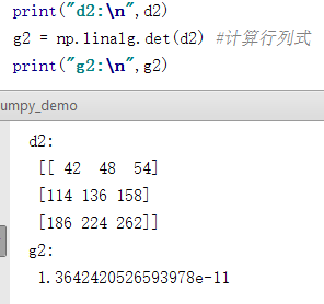
trace 计算对角线元素的和
det 计算矩阵行列式
eig 计算方阵的特征值和特征向量
inv 计算方阵的逆

在这里插入图片描述

Numpy保存和导入文件

Numpy提供了save和load接口，直接将数组保存成文件(保存为.npy格式)，或者从.npy文件中读取数组:

def method_2():
    a2 = np.random.rand(3,3)
    print("a2:\n",a2)
    np.save('a.npy', a2)
    b2 = np.load('a.npy')
    print("b2:\n",b2)

在这里插入图片描述
下面是AI Studio上的应用举例:

Numpy应用举例1——计算激活函数

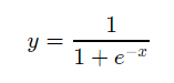
使用ndarray数组可以很方便的构建数学函数，而且能利用其底层的矢量计算能力快速实现计算。神经网络中比较常用激活函数是Sigmoid和ReLU，其定义如下

Sigmoid激活函数:
在这里插入图片描述
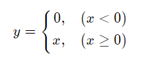
ReLU激活函数:

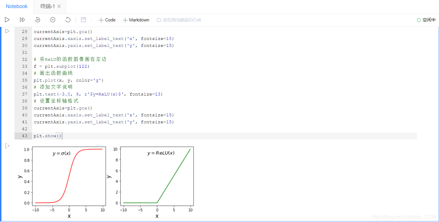
下面使用numpy和matplotlib计算函数值并画出图形:

# ReLU和Sigmoid激活函数示意图
import numpy as np
%matplotlib inline
import matplotlib.pyplot as plt
import matplotlib.patches as patches

#设置图片大小
plt.figure(figsize=(8, 3))

# x是1维数组，数组大小是从-10. 到10.的实数，每隔0.1取一个点
x = np.arange(-10, 10, 0.1)
# 计算 Sigmoid函数
s = 1.0 / (1 + np.exp(- x))

# 计算ReLU函数
y = np.clip(x, a_min = 0., a_max = None)

#########################################################
# 以下部分为画图程序

# 设置两个子图窗口，将Sigmoid的函数图像画在左边
f = plt.subplot(121)
# 画出函数曲线
plt.plot(x, s, color='r')
# 添加文字说明
plt.text(-5., 0.9, r'$y=\sigma(x)$', fontsize=13)
# 设置坐标轴格式
currentAxis=plt.gca()
currentAxis.xaxis.set_label_text('x', fontsize=15)
currentAxis.yaxis.set_label_text('y', fontsize=15)

# 将ReLU的函数图像画在左边
f = plt.subplot(122)
# 画出函数曲线
plt.plot(x, y, color='g')
# 添加文字说明
plt.text(-3.0, 9, r'$y=ReLU(x)$', fontsize=13)
# 设置坐标轴格式
currentAxis=plt.gca()
currentAxis.xaxis.set_label_text('x', fontsize=15)
currentAxis.yaxis.set_label_text('y', fontsize=15)

plt.show()

在这里插入图片描述
Numpy应用举例2——图像翻转和裁剪

图像是由像素点构成的矩阵，其数值可以用ndarray来表示:

import numpy as np
import matplotlib.pyplot as plt
from PIL import Image
# 读入图片
image = Image.open('2007_003267.jpg')
image = np.array(image)
# 查看数据形状，其形状是[H, W, 3]，
# 其中H代表高度， W是宽度，3代表RGB三个通道
image.shape

在这里插入图片描述

image2 = image[::-1, :, :]
plt.imshow(image2)

垂直方向翻转,这里使用数组切片的方式来完成，相当于将图片最后一行挪到第一行，倒数第二行挪到第二行，…, 第一行挪到倒数第一行,对于行指标，使用::-1来表示切片，负数步长表示以最后一个元素为起点，向左走寻找下一个点,对于列指标和RGB通道，仅使用:表示该维度不改变
在这里插入图片描述

# 水平方向翻转
image3 = image[:, ::-1, :]
plt.imshow(image3)

在这里插入图片描述

# 保存图片
im3 = Image.fromarray(image3)
im3.save('im3.jpg')

在这里插入图片描述

#  高度方向裁剪
H, W = image.shape[0], image.shape[1]
# 注意此处用整除，H_start必须为整数
H1 = H // 2 
H2 = H
image4 = image[H1:H2, :, :]
plt.imshow(image4)

在这里插入图片描述

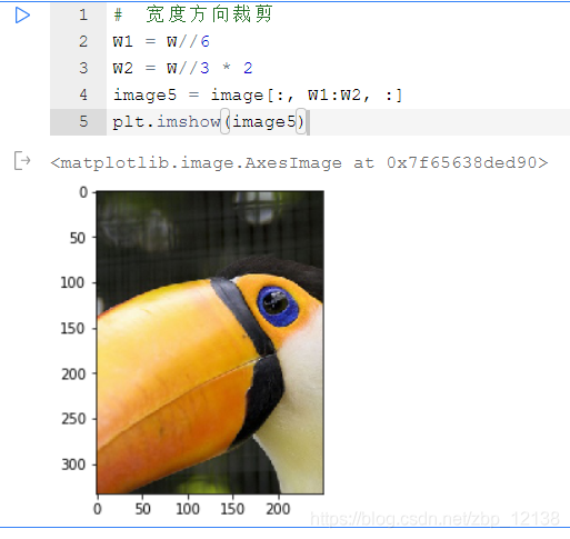
#  宽度方向裁剪
W1 = W//6
W2 = W//3 * 2
image5 = image[:, W1:W2, :]
plt.imshow(image5)

在这里插入图片描述

# 两个方向同时裁剪
image5 = image[H1:H2, \
               W1:W2, :]
plt.imshow(image5)

在这里插入图片描述

# 调整亮度
image6 = image * 0.5
plt.imshow(image6.astype('uint8'))

在这里插入图片描述

# 调整亮度
image7 = image * 2.0
# 由于图片的RGB像素值必须在0-255之间，
# 此处使用np.clip进行数值裁剪
image7 = np.clip(image7, \
        a_min=None, a_max=255.)
plt.imshow(image7.astype('uint8'))

在这里插入图片描述

#高度方向每隔一行取像素点
image8 = image[::2, :, :]
plt.imshow(image8)

在这里插入图片描述

#宽度方向每隔一列取像素点
image9 = image[:, ::2, :]
plt.imshow(image9)

在这里插入图片描述

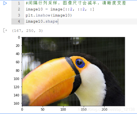
#间隔行列采样，图像尺寸会减半，清晰度变差
image10 = image[::2, ::2, :]
plt.imshow(image10)
image10.shape

在这里插入图片描述
tanh也是神经网络中常用的一种激活函数,下面我们使用numpy计算tanh激活函数:

import numpy as np
import matplotlib.pyplot as plt

#设置图片大小
plt.figure(figsize=(8, 3))

# x是1维数组，数组大小是从-10. 到10.的实数，每隔0.1取一个点
x = np.arange(-10, 10, 0.1)
# 计算 tanh函数
t = (np.exp(x) - np.exp(- x)) / (np.exp(x) + np.exp(- x))

# 画出函数曲线
plt.plot(x, t, color='r')
# 添加文字说明
plt.text(-5., 0.9, r'$y=\tanh(x)$', fontsize=13)
# 设置坐标轴格式
currentAxis=plt.gca()
currentAxis.xaxis.set_label_text('x', fontsize=15)
currentAxis.yaxis.set_label_text('y', fontsize=15)

plt.show()

在这里插入图片描述
下面,我们统计一下随机生成矩阵中有多少个元素大于0:

这里我用了最简单的方法,即使用两个for循环

import numpy as np

arr = np.random.randn(10,10)
print(arr)
arr[arr < 0] = 0
print(arr)
resdata = []
for i in range(len(arr)):
    for j in range(len(arr)):
        if arr[i][j] > 0:
            resdata.append(arr[i][j])
print(len(resdata))

在这里插入图片描述
当然,这里肯定还有更加便捷的算法,欢迎大家在评论区交流讨论!

Mr.郑先生_

发布了60 篇原创文章 · 获赞 123 · 访问量 4万+

私信关注

一篇文章搞懂Numpy的Python学习指北(文末附应用举例)

猜你喜欢