python—skimage examples（1）

参考网站在这里

1.绘制两个子图

补充知识：
Python 字典(Dictionary)
什么是rcParams
plt.tight_layout()的作用

import numpy as np
import matplotlib.pyplot as plt
import matplotlib

from skimage import data

matplotlib.rcParams['font.size']=18
#RcParams用于修改matplotlib默认值。
fig,axes=plt.subplots(1,2,figsize=(8,4))
ax=axes.ravel()#??
images=data.stereo_motorcycle() #skimage自带图库
ax[0].imshow(images[0])
ax[1].imshow(images[1])
fig.tight_layout()
#tight_layout会自动调整子图参数，使之填充整个图像区域
plt.show()

2.绘制多个子图

补充知识：
numpy 中降维函数ravel（）
理解 Python 的 for 循环
subplot() subplots()的区别与使用

import numpy as np
import matplotlib.pyplot as plt
import matplotlib
from skimage import data
matplotlib.rcParams['font.size']=18

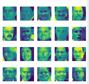
fig,axes=plt.subplots(4,5,figsize=(20,20))
ax=axes.ravel() #将多维数组拉平（一维）
images=data.lfw_subset()
# LFW (Labled Faces in the Wild)人脸数据集:是目前人脸识别的常用测试集
for i in range(20):
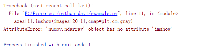
    ax[i].imshow(images[20+i],cmap=plt.cm.gray)#使用自定义的colormap（灰度图）
    ax[i].axis('off')

fig.tight_layout()
#tight_layout会自动调整子图参数，使之填充整个图像区域
plt.show()

不太明白为什么是这个画质
思考1：如果不添加 ax=axes.ravel()，就会出现如下错误
因为for i in range(20): 只用了一层循环，否则要用2曾循环遍历axes[]数组

思考2：如果删除,cmap=plt.cm.gray，图片会变成

3 调用skimage自带图片

补充知识：
getattr 内置函数

import matplotlib.pyplot as plt
import matplotlib
from skimage import data

matplotlib.rcParams['font.size']=18
#The title of each image indicates the name of the function.
images=('hubble_deep_field',
        'immunohistochemistry',
        'microaneurysms',
        'moon',
        'retina',
        )
for name in images:
    caller=getattr(data,name)
    image=caller()
    plt.figure()
    plt.title(name)
    plt.imshow(image)
plt.show()

逐张显示

4 使用简单的NumPy操作来处理图像

补充知识：
pycharm 下如何调试python
range 和arange的区别
numpy的ogrid详细介绍
Python 数组，字典，元组，集合

import matplotlib.pyplot as plt
import numpy as np
from skimage import data

camera=data.camera()  #camera 是ndarray 的数组
camera[:10]=0    #将 0-9行置为0
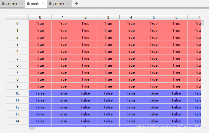
mask=camera<87  # ‘< ’为条件语句，只能返回“真假”。将camera中像素值<87的位置记为true,其余为false
camera[mask]=255    #再利用mask所标记的位置（true和false）,将值为true 的值设为255
inds_x=np.arange(len(camera))  #   inds_x 秩为1 的数组 ：inds_x.shape=(512,)，记录camera的横坐标0~511
inds_y=(4*inds_x)%len(camera)   #   inds_y秩为1 的数组,记录 经过处理后的纵坐标
camera[inds_x,inds_y]=0     # 按一定规律将像素置为零

l_x,l_y=camera.shape[0],camera.shape[1]  # 512 ，512
X,Y=np.ogrid[:l_x,:l_y]
outer_disk_mask=(X-l_x/2)**2+(Y-l_y/2)**2>(l_x/2)**2
# 注意该赋值号右边有条件语句‘>’ ,所以返回的是真假(true/false)
camera[outer_disk_mask]=0

plt.figure(figsize=(4,4))
plt.imshow(camera,cmap='gray')
plt.axis('off')
plt.show()

结果：

分析：
可以通过调试，查看变量类型。

camera[:10]=0 的可视化
mask=camera<87
mask 是只存true和false的矩阵，将camera中像素值<87的位置记为true,其余为false
camera[mask]=255
再利用mask所标记的位置（true和false）,将值为true 的值设为255.于是得到下图（第一张为mask,第二张为camera）

扫描二维码关注公众号，回复： 10300186 查看本文章

5.Block views on images

对不重叠的图像块执行局部操作（不是很理解其作用）

import numpy as np
from scipy import ndimage as ndi
from matplotlib import pyplot as plt
import matplotlib.cm as cm
from skimage import data
from skimage import color
from skimage.util import view_as_blocks

#get astronaut from skimage.data in grayscale
l=color.rgb2gray(data.astronaut())      #<class 'tuple'>: (512, 512) #转灰度图
#size of blocks
block_shape=(4,4)
#see astronaut as a matrix of blocks(of shape block_shape)
view=view_as_blocks(l,block_shape)  #<class 'tuple'>: (128, 128, 4, 4)

#collapse the last two dimensions in one
flatten_view=view.reshape(view.shape[0],view.shape[1],-1)  #<class 'tuple'>: (128, 128, 16)

#resampling the image
mean_view=np.mean(flatten_view,axis=2)  #<class 'tuple'>: (128, 128)
max_view=np.max(flatten_view,axis=2)
median_view=np.median(flatten_view,axis=2)      #中值

#display reshaped images
fig,axes=plt.subplots(2,2,figsize=(8,8),sharex=True,sharey=True)
ax=axes.ravel()

#l_resized=ndi.zoom(1,2,order=3)      #样条插值
ax[0].set_title("Original")
ax[0].imshow(l,cmap=cm.Greys_r)
ax[1].set_title("local mean pooling")
ax[1].imshow(mean_view,cmap=cm.Greys_r)
ax[2].set_title("local max pooling")
ax[2].imshow(max_view,cmap=cm.Greys_r)
ax[3].set_title("local median pooling")
ax[3].imshow(median_view,cmap=cm.Greys_r)

for a in ax:
    a.set_axis_off()
fig.tight_layout()
plt.show()

6.RGB to HSV

补充知识：

1. HSV:色调（H），饱和度（S），明度（V）
2. 从 RGB 到 HSV 的转换详细介绍
3. 例子：
   pixel=img[20,30,1] #G通道中的第20行30列的像素值
   img[:,:,0] #R通道所有像素值

import matplotlib.pyplot as plt
from skimage import data
from skimage.color import rgb2hsv
from skimage import io

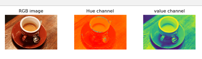
#加载RGB图像，并提取色相和值通道
rgb_img=data.coffee()
#io.imshow(rgb_img)
#plt.show()
hsv_img=rgb2hsv(rgb_img)
hue_img=hsv_img[:,:,0]
value_img=hsv_img[:,:,2]
fig,ax=plt.subplots(1,3,figsize=(8,2))
ax[0].imshow(rgb_img)
ax[0].set_title("RGB image")
ax[0].axis('off')
ax[1].imshow(hue_img,cmap='hsv')
ax[1].set_title("Hue channel")
ax[1].axis('off')
ax[2].imshow(value_img)
ax[2].set_title("value channel")
ax[2].axis('off')
fig.tight_layout()
plt.show()

#然后，在色相通道熵设置一个阈值，将杯子与背景分开                                                                  
rgb_img=data.coffee()                                                                      
hsv_img=rgb2hsv(rgb_img)                                                                   
hue_img=hsv_img[:,:,0]                                                                     
value_img=hsv_img[:,:,2]                                                                   
hue_threshold=0.04                                                                         
binary_img=hue_img>hue_threshold                                                           
                                                                                           
fig,ax=plt.subplots(1,2,figsize=(8,3))                                                     
ax[0].hist(hue_img.ravel(),512)                                                            
ax[0].set_title("Histogram of the Hue channel with threshold")                             
ax[0].axvline(x=hue_threshold,color='r',linestyle='dashed',linewidth=2)                    
ax[0].set_xbound(0,0.12)                                                                   
ax[1].imshow(binary_img)                                                                   
ax[1].set_title("Hue-thresholded image")                                                   
ax[1].axis('off')                                                                          
fig.tight_layout()                                                                         
plt.show()                                                                                 

#最后，在value通道处加阈值处理  ,除去杯子的阴影                                          
rgb_img=data.coffee()                                                 
hsv_img=rgb2hsv(rgb_img)                                              
hue_img=hsv_img[:,:,0]                                                
value_img=hsv_img[:,:,2]                                              
hue_threshold=0.04                                                    
value_threshold=0.01                                                  
binary_img=(hue_img>hue_threshold)|(value_img<value_threshold)        
                                                                      
fig,ax0=plt.subplots(figsize=(4,3))                                   
ax0.imshow(binary_img)                                                
ax0.set_title("hue and value thresholded image")                      
ax0.axis('off')                                                       
fig.tight_layout()                                                    
plt.show()                                                            
                                                                      

7.直方图匹配

准备知识：
直方图均衡

import numpy as np
from skimage import exposure,data
img=data.camera()*0.1
hist1=np.histogram(img,bins=2) #使用numpy包计算直方图
hist2=exposure.histogram(img,nbins=2)#用skimage计算直方图
print(hist1)
print(hist2)

结果

(array([107432, 154712], dtype=int64), array([ 0.  , 12.75, 25.5 ]))
(array([107432, 154712], dtype=int64), array([ 6.375, 19.125]))

绘制直方图

n, bins, patches = plt.hist(arr, bins=10, normed=0, facecolor='black', edgecolor='black',alpha=1，histtype='bar')

参数：

arr: 需要计算直方图的一维数组
bins: 直方图的柱数，可选项，默认为10
normed: 是否将得到的直方图向量归一化。默认为0
facecolor: 直方图颜色
edgecolor: 直方图边框颜色
alpha: 透明度
histtype: 直方图类型，‘bar’, ‘barstacked’, ‘step’, ‘stepfilled’

返回值：

n: 直方图向量，是否归一化由参数normed设定
bins: 返回各个bin的区间范围
patches: 返回每个bin里面包含的数据，是一个list

import numpy as np
from skimage import exposure,data
import matplotlib.pyplot as plt

img=data.coffee()
plt.figure("hist")
arr=img.flatten()
#其中的flatten()函数是numpy包里面的，用于将二维数组序列化成一维数组。
n,bins,patches=plt.hist(arr,bins=256,normed=1,edgecolor='None',facecolor='red')
plt.show()

直方图均衡化

from skimage import exposure,data
import matplotlib.pyplot as plt

img=data.moon()
plt.figure("hist",figsize=(8,8))

arr=img.flatten()
plt.subplot(221)
plt.imshow(img,plt.cm.gray)
plt.subplot(222)
plt.hist(arr,bins=265,normed=1,edgecolor='None',facecolor='red')

img1=exposure.equalize_hist(img)
arr1=img1.flatten()
plt.subplot(223)
plt.imshow(img1,plt.cm.gray)
plt.subplot(224)
plt.hist(arr1,bins=256,normed=1,edgecolor='None',facecolor='red')
plt.show()

1.transform

from skimage import transform,data
import matplotlib.pyplot as plt
#resize改变图片尺寸
img=data.coffee()
dst=transform.resize(img,(80,60))
plt.figure('resize')

plt.subplot(121)
plt.title('before resize')
plt.imshow(img,plt.cm.gray)

plt.subplot(122)
plt.title('after resize')
plt.imshow(dst,plt.cm.gray)

plt.show()

from skimage import transform,data
import matplotlib.pyplot as plt

#rotate 旋转

#skimage.transform.rotate(image, angle[, ...],resize=False)
#angle参数是个float类型数，表示旋转的度数
#resize用于控制在旋转时，是否改变大小 ，默认为False

img=data.coffee()
img1=transform.rotate(img,60)#旋转60°，不改变大小
img2=transform.rotate(img,30,resize=True)#旋转60°，改变大小
print(img.shape)
print(img1.shape)
print(img2.shape)

fig,ax=plt.subplots(1,3)
ax[0].imshow(img)
ax[0].set_title("Original")
ax[0].axis('off')
ax[1].imshow(img1)
ax[1].set_title("rotate 60")
ax[1].axis('off')
ax[2].imshow(img2)
ax[2].set_title("rotate 30")
ax[2].axis('off')

fig.tight_layout()
plt.show()

结果：
(400, 600, 3)
(400, 600, 3)
(647, 720, 3)

2.图像简单滤波

图像滤波分为两种：平滑滤波（除噪），微分算子（检测边缘，提取特征）

sobel算子

from skimage import filters,data
import matplotlib.pyplot as plt
img=data.camera()
edges=filters.sobel(img)
plt.imshow(edges,plt.cm.gray)
plt.show()

roberts，scharr，prewitt等算子与sobel算子功能类似

3.插值算法

帮助：
最近邻插值、双线性插值、双三次插值