MLE v.s. MAP ~ L1, L2 Math Derivation 详细

MLE v.s. MAP

• MLE: learn parameters from data.
• MAP: add a prior (experience) into the model; more reliable if data is limited. As we have more and more data, the prior becomes less useful.
• As data increase, MAP $\rightarrow$ MLE.

Notation: $D = \{(x_1, y_1), (x_2, y_2), ..., (x_n, y_n)\}$

Framework:

• MLE: $\mathop{\rm arg\,max} P(D \,|\, \theta)$
• MAP: $\mathop{\rm arg\,max} P(\theta \,|\, D)$

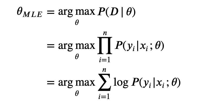
Note that taking a product of some numbers less than 1 would approaching 0 as the number of those numbers goes to infinity, it would be not practical to compute, because of computation underflow. Hence, we will instead work in the log space.

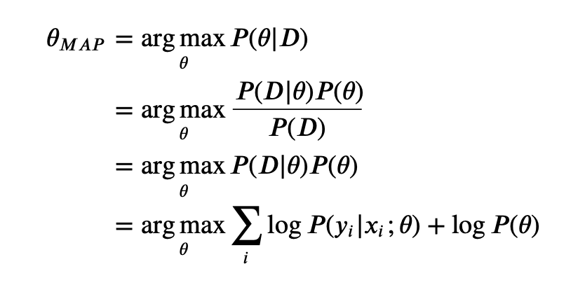
Comparing both MLE and MAP equation, the only thing differs is the inclusion of prior
$P(\theta)$ in MAP, otherwise they are identical. What it means is that, the likelihood is now weighted with some weight coming from the prior.

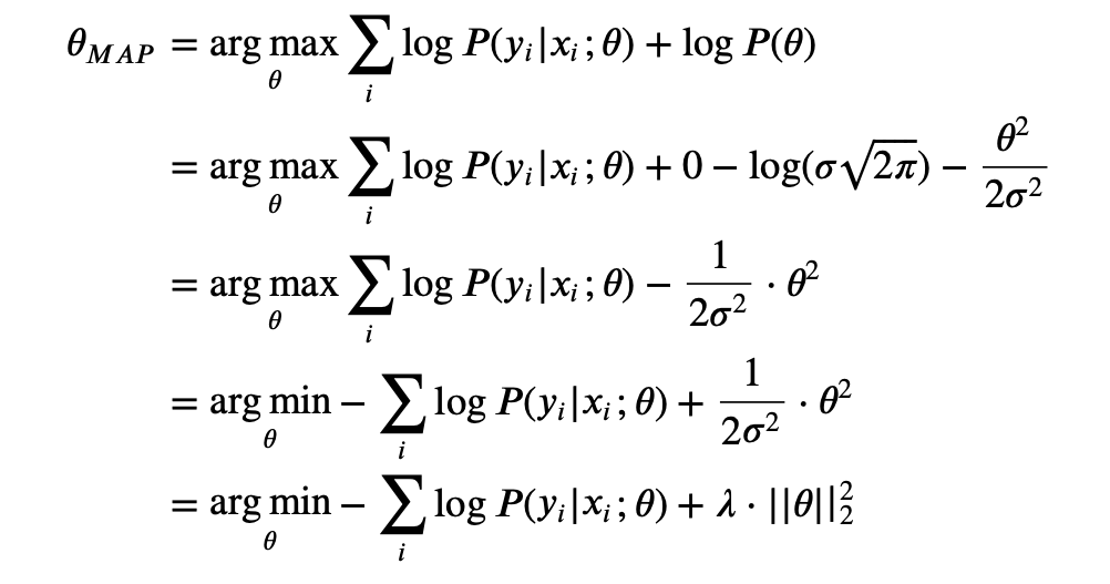
If the prior follows the normal distribution, then it is the same as adding a $L2$ regularization.

We assume $P(\theta) \sim \mathcal{N}(0, \sigma^2)$, then $P(x) = \frac{1}{\sigma \sqrt {2\pi}}exp(-\frac{\theta^2}{2\sigma^2})$

If the prior follows the Laplace distribution, then it is the same as adding a $L1$ regularization.

We assume $P(\theta) \sim Laplace \,(\mu=0, b)$, then $P(\theta) = \frac{1}{2b}exp(-\frac{|\theta|}{b})$