【数据分析】数据挖掘-3

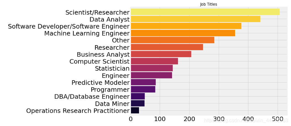
看看数据科学家们做什么

plt.subplots(figsize=(10,8))
scientist=response[response['DataScienceIdentitySelect']=='Yes']
scientist['CurrentJobTitleSelect'].value_counts().sort_values(ascending=True).plot.barh(width=0.9,color=sns.color_palette('inferno',15))
plt.title('Job Titles',size=15)
plt.show()

教育背景以及工作情况

f,ax=plt.subplots(1,2,figsize=(25,10))
sns.countplot(y=scientist['EmploymentStatus'],ax=ax[0])
ax[0].set_title('Employment Status')
ax[0].set_ylabel('')
sns.countplot(y=scientist['FormalEducation'],order=scientist['FormalEducation'].value_counts().index,ax=ax[1],palette=sns.color_palette('viridis_r',15))
ax[1].set_title('Formal Eduaction')
ax[1].set_ylabel('')
plt.subplots_adjust(wspace=0.8)
plt.show()

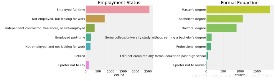
大约67%的数据科学家都是全职，而大约11-12%都失业而找工作。在教育方面显然对76 %的数据科学家持有硕士学位，而约23-24%他们有学士学位或博士学位。因此，教育似乎是成为数据科学家的一个重要因素。让我们看看工资是如何根据教育而变化的。

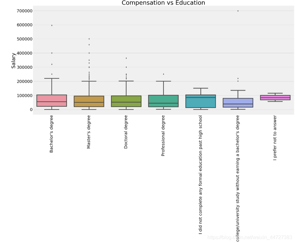
学历跟工资

plt.subplots(figsize=(25,12))
comp_edu=scientist.merge(salary,left_index=True,right_index=True,how='left')
comp_edu=comp_edu[['FormalEducation','Salary']]
sns.boxplot(x='FormalEducation',y='Salary',data=comp_edu)
plt.title('Compensation vs Education')
plt.xticks(rotation=90)
plt.show()

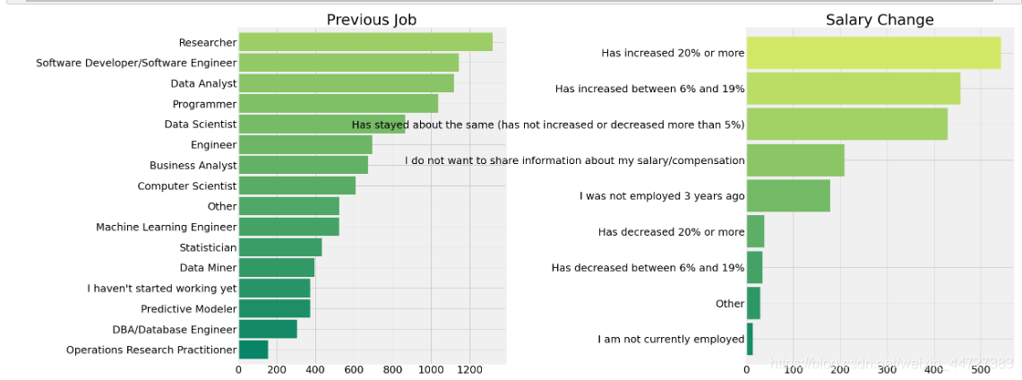
前一份工作和现在的改变

f,ax=plt.subplots(1,2,figsize=(30,15))
past=scientist['PastJobTitlesSelect'].str.split(',')
past_job=[]
for i in past.dropna():
    past_job.extend(i)
pd.Series(past_job).value_counts().sort_values(ascending=True).plot.barh(width=0.9,color=sns.color_palette('summer',25),ax=ax[0])
ax[0].set_title('Previous Job')
sal=scientist['SalaryChange'].str.split(',')
sal_change=[]
for i in sal.dropna():
    sal_change.extend(i)
pd.Series(sal_change).value_counts().sort_values(ascending=True).plot.barh(width=0.9,color=sns.color_palette('summer',10),ax=ax[1])
ax[1].set_title('Salary Change')
plt.subplots_adjust(wspace=0.9)
plt.show()

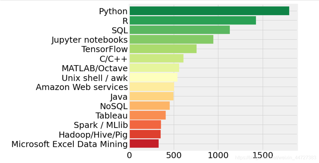
数据科学家们都用什么

plt.subplots(figsize=(8,8))
tools=scientist['WorkToolsSelect'].str.split(',')
tools_work=[]
for i in tools.dropna():
    tools_work.extend(i)
pd.Series(tools_work).value_counts()[:15].sort_values(ascending=True).plot.barh(width=0.9,color=sns.color_palette('RdYlGn',15))
plt.show()

他们都在哪学习

course=scientist['CoursePlatformSelect'].str.split(',')
course_plat=[]
for i in course.dropna():
    course_plat.extend(i)
course_plat=pd.Series(course_plat).value_counts()
blogs=scientist['BlogsPodcastsNewslettersSelect'].str.split(',')
blogs_fam=[]
for i in blogs.dropna():
    blogs_fam.extend(i)
blogs_fam=pd.Series(blogs_fam).value_counts()
labels1=course_plat.index
sizes1=course_plat.values

labels2=blogs_fam[:5].index
sizes2=blogs_fam[:5].values


fig = {
  "data": [
    {
      "values": sizes1,
      "labels": labels1,
      "domain": {"x": [0, .48]},
      "name": "MOOC",
      "hoverinfo":"label+percent+name",
      "hole": .4,
      "type": "pie"
    },     
    {
      "values": sizes2 ,
      "labels": labels2,
      "text":"CO2",
      "textposition":"inside",
      "domain": {"x": [.54, 1]},
      "name": "Blog",
      "hoverinfo":"label+percent+name",
      "hole": .4,
      "type": "pie"
    }],
  "layout": {
        "title":"Blogs and Online Platforms",
        "showlegend":True,
        "annotations": [
            {
                "font": {
                    "size": 12
                },
                "showarrow": False,
                "text": "MOOC's",
                "x": 0.18,
                "y": 0.5
            },
            {
                "font": {
                    "size": 12
                },
                "showarrow": False,
                "text": "BLOGS",
                "x": 0.83,
                "y": 0.5}]}}
py.iplot(fig, filename='donut')

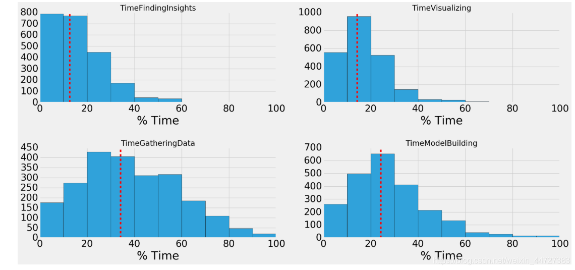
时间都去哪了

import itertools
plt.subplots(figsize=(22,10))
time_spent=['TimeFindingInsights','TimeVisualizing','TimeGatheringData','TimeModelBuilding']
length=len(time_spent)
for i,j in itertools.zip_longest(time_spent,range(length)):
    plt.subplot((length/2),2,j+1)
    plt.subplots_adjust(wspace=0.2,hspace=0.5)
    scientist[i].hist(bins=10,edgecolor='black')
    plt.axvline(scientist[i].mean(),linestyle='dashed',color='r')
    plt.title(i,size=20)
    plt.xlabel('% Time')
plt.show()

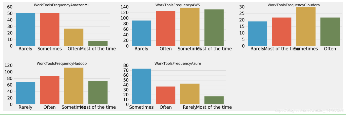
常用平台

cloud=['WorkToolsFrequencyAmazonML','WorkToolsFrequencyAWS','WorkToolsFrequencyCloudera','WorkToolsFrequencyHadoop','WorkToolsFrequencyAzure']
plt.subplots(figsize=(30,15))
length=len(cloud)
for i,j in itertools.zip_longest(cloud,range(length)):
    plt.subplot((length/2+1),3,j+1)
    plt.subplots_adjust(wspace=0.2,hspace=0.5)
    sns.countplot(i,data=scientist)
    plt.title(i,size=20)
    plt.ylabel('')
    plt.xlabel('')
plt.show()

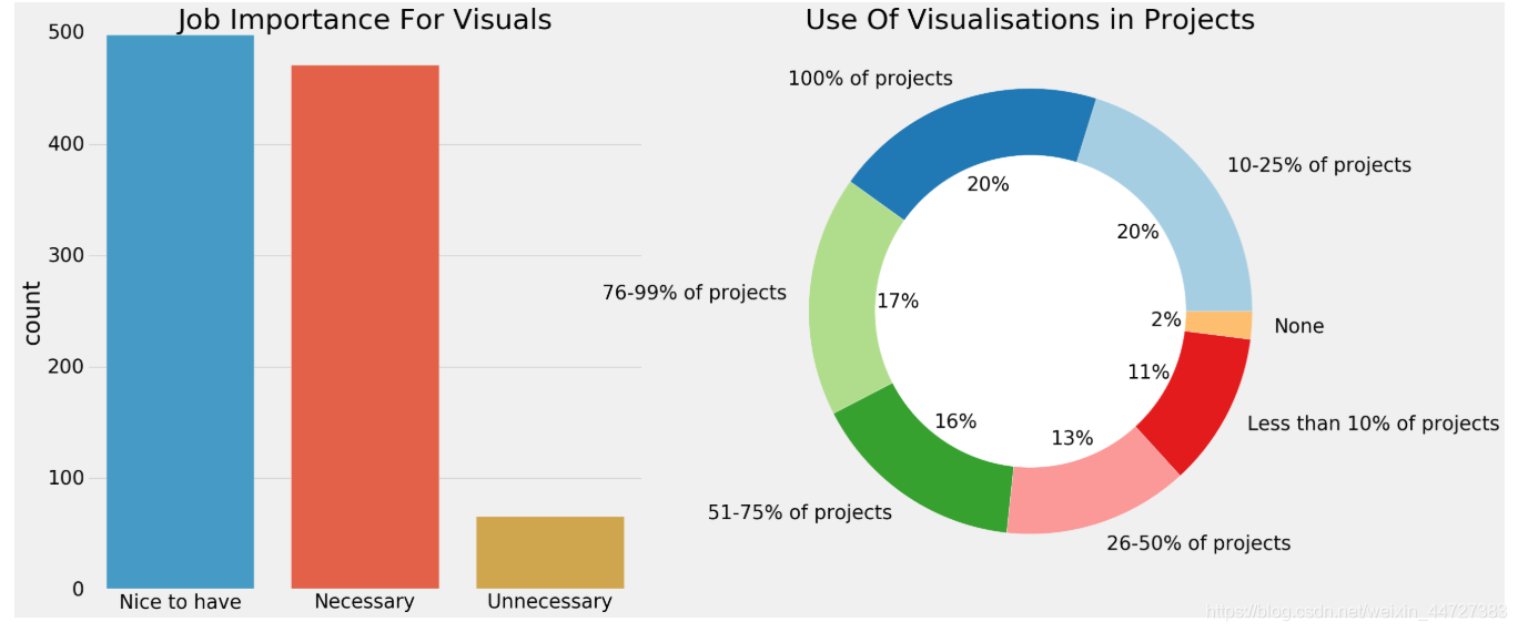
对可视化的重视程度

f,ax=plt.subplots(1,2,figsize=(25,12))
sns.countplot(scientist['JobSkillImportanceVisualizations'],ax=ax[0])
ax[0].set_title('Job Importance For Visuals')
ax[0].set_xlabel('')
scientist['WorkDataVisualizations'].value_counts().plot.pie(autopct='%2.0f%%',colors=sns.color_palette('Paired',10),ax=ax[1])
ax[1].set_title('Use Of Visualisations in Projects')
my_circle=plt.Circle( (0,0)a, 0.7, color='white')
p=plt.gcf()
p.gca().add_artist(my_circle)
plt.ylabel('')
plt.show()

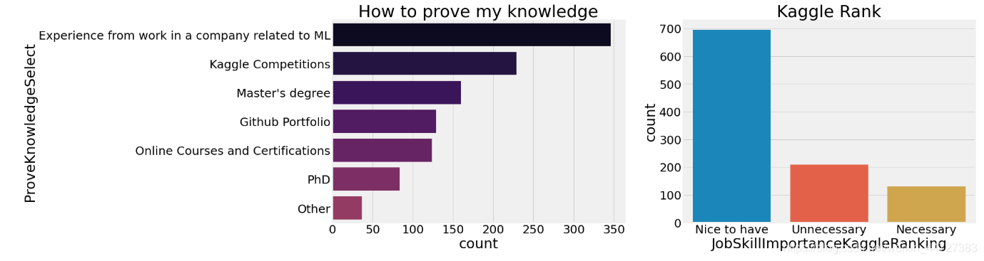
如何证明你的实力

f,ax=plt.subplots(1,2,figsize=(22,8))
sns.countplot(y=scientist['ProveKnowledgeSelect'],order=scientist['ProveKnowledgeSelect'].value_counts().index,ax=ax[0],palette=sns.color_palette('inferno',15))
ax[0].set_title('How to prove my knowledge')
sns.countplot(scientist['JobSkillImportanceKaggleRanking'],ax=ax[1])
ax[1].set_title('Kaggle Rank')
plt.show()

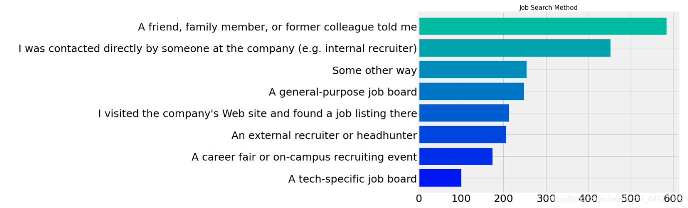
怎么找工作

plt.subplots(figsize=(10,8))
scientist.groupby(['EmployerSearchMethod'])['Age'].count().sort_values(ascending=True).plot.barh(width=0.8,color=sns.color_palette('winter',10))
plt.title('Job Search Method',size=15)
plt.ylabel('')
plt.show()

在Python和R中最常用什么

import nltk


stopwords=nltk.download('stopwords')
stop_words=set(stopwords.words('english'))
stop_words.update(',',';','!','?','.','(',')','$','#','+',':','...')

free=pd.read_csv('freeformResponses.csv',encoding='ISO-8859-1')
library=free['WorkLibrariesFreeForm'].dropna().apply(nltk.word_tokenize)
lib=[]
for i in library:
    lib.extend(i)
lib=pd.Series(lib)
lib=([i for i in lib.str.lower() if i not in stop_words])
lib=pd.Series(lib)
lib=lib.value_counts().reset_index()
lib.loc[lib['index'].str.contains('Pandas|pandas|panda'),'index']='Pandas'
lib.loc[lib['index'].str.contains('Tensorflow|tensorflow|tf|tensor'),'index']='Tensorflow'
lib.loc[lib['index'].str.contains('Scikit|scikit|sklearn'),'index']='Sklearn'
lib=lib.groupby('index')[0].sum().sort_values(ascending=False).to_frame()
R_packages=['dplyr','tidyr','ggplot2','caret','randomforest','shiny','R markdown','ggmap','leaflet','ggvis','stringr','tidyverse','plotly']
Py_packages=['Pandas','Tensorflow','Sklearn','matplotlib','numpy','scipy','seaborn','keras','xgboost','nltk','plotly']
f,ax=plt.subplots(1,2,figsize=(18,10))
lib[lib.index.isin(Py_packages)].sort_values(by=0,ascending=True).plot.barh(ax=ax[0],width=0.9,color=sns.color_palette('viridis',15))
ax[0].set_title('Most Frequently Used Py Libraries')
lib[lib.index.isin(R_packages)].sort_values(by=0,ascending=True).plot.barh(ax=ax[1],width=0.9,color=sns.color_palette('viridis',15))
ax[1].set_title('Most Frequently Used R Libraries')
ax[1].set_ylabel('')
plt.show()

结论:

1）大多数受访者来自美国.

2）大多数的受访者在年龄20-35岁，这表明数据科学的年轻人是很著名的。

3）调查对象不仅限于计算机科学专业，还包括统计学、健康科学等专业，数据科学是一门跨学科的领域。

4）大多数被调查者都被充分雇用。

5）Kaggle，在线课程（Coursera，edX，等），项目和博客（kdnuggets，analyticsvidya，等）是学习数据科学的首选资源。

6）Kaggle数据采集与GitHub的代码共享是大家非常喜欢的

7）数据科学家的工作满意度最高，相反程序员的工作满意度最低。

8）数据科学家也从以前的工作中获得的提升大约6～20%。

1）学习Python、R和SQL，因为它们是数据科学家最常用的语言。Python和R将有助于分析和预测建模，而SQL最适合查询数据库。

2）学习机器学习技术，如逻辑回归，决策树，支持向量机等，因为它们是最常用的机器学习技术/算法。

3）深学习和神经网络将是未来最受欢迎的技术，因此，精通它们将是非常有益的。

4）掌握收集数据和清理数据的技能，因为它们是数据科学家工作流程中最耗时的过程。

5）可视化是非常重要的数据科学项目以及几乎所有的项目都需要了解数据的可视化。

6）数学和统计在数据科学中是非常重要的，所以我们应该对它有很好的理解，以便真正理解算法是如何工作的。

7）根据数据科学家们说，项目是学习数据科学的最佳途径，因此，研究项目将有助于更好地学习数据科学。