TensorFlow基础系列（神经网络NN）

开篇

算起凌晨的那一篇词袋模型，这是今天的第三篇TensorFlow博客，我们也要开始跑一点真实的数据集啦。不能总是拿着自己随便捏造的一点数据来描述我们的算法，可能会有点老套，但是我还是决定选择一个比较常被用用到的数据集，手写数字的数据集。找了一大圈数据集的下载，发现在csdn上还需要积分下载，这种本来就应该是免费下载使用的数据集还要积分就有点过分啦。这里放上我的下载链接链接:https://pan.baidu.com/s/1TXvTbX59OF_rAi-ye6wYQQ 密码:6fu6。大家下载的时候记得修改一些数据集的名字，我直接用的temp为名的，但是下面的代码中使用的是MNIST_data命名的。OK，废话不多说，下面马上开始我们的正式内容。

任务

简单的说一下我们今天要处理的任务，我会分别使用softmax和nn来处理我们的任务，会有两个完整的代码，后期我们还会使用cnn来处理我们的任务。使用的数据集是手写数字，那么我们要做的任务就是手写数字识别，说白了也就是我们的多分类任务，给一张手写的数字图片，我们给出它正确的数字类别。首先我们使用单纯的softmax去实现，也弥补一下我们上篇博客没有使用真实的数据集的遗憾。

代码

扯了半天该上我们的代码了，首先是softmax的完整代码

# Lab 7 Learning rate and Evaluation
import tensorflow as tf
import random
# import matplotlib.pyplot as plt
from tensorflow.examples.tutorials.mnist import input_data
tf.set_random_seed(777)  # reproducibility

mnist = input_data.read_data_sets("MNIST_data/", one_hot=True)
# Check out https://www.tensorflow.org/get_started/mnist/beginners for
# more information about the mnist dataset

# parameters
learning_rate = 0.001
training_epochs = 15
batch_size = 100

# input place holders
X = tf.placeholder(tf.float32, [None, 784])
Y = tf.placeholder(tf.float32, [None, 10])

# weights & bias for nn layers
W = tf.Variable(tf.random_normal([784, 10]))
b = tf.Variable(tf.random_normal([10]))

hypothesis = tf.matmul(X, W) + b

# define cost/loss & optimizer
cost = tf.reduce_mean(tf.nn.softmax_cross_entropy_with_logits(
    logits=hypothesis, labels=Y))
optimizer = tf.train.AdamOptimizer(learning_rate=learning_rate).minimize(cost)

# initialize
sess = tf.Session()
sess.run(tf.global_variables_initializer())

# train my model
for epoch in range(training_epochs):
    avg_cost = 0
    total_batch = int(mnist.train.num_examples / batch_size)

    for i in range(total_batch):
        batch_xs, batch_ys = mnist.train.next_batch(batch_size)
        feed_dict = {X: batch_xs, Y: batch_ys}
        c, _ = sess.run([cost, optimizer], feed_dict=feed_dict)
        avg_cost += c / total_batch

    print('Epoch:', '%04d' % (epoch + 1), 'cost =', '{:.9f}'.format(avg_cost))

print('Learning Finished!')

# Test model and check accuracy
correct_prediction = tf.equal(tf.argmax(hypothesis, 1), tf.argmax(Y, 1))
accuracy = tf.reduce_mean(tf.cast(correct_prediction, tf.float32))
print('Accuracy:', sess.run(accuracy, feed_dict={
      X: mnist.test.images, Y: mnist.test.labels}))

# Get one and predict
r = random.randint(0, mnist.test.num_examples - 1)
print("Label: ", sess.run(tf.argmax(mnist.test.labels[r:r + 1], 1)))
print("Prediction: ", sess.run(
    tf.argmax(hypothesis, 1), feed_dict={X: mnist.test.images[r:r + 1]}))

# plt.imshow(mnist.test.images[r:r + 1].
#           reshape(28, 28), cmap='Greys', interpolation='nearest')
# plt.show()

到这里基本上就牵出了我们深度学习中几个比较重要的概念，和模型的训练有关。
首先是batchsize，在我们深度学习的模型训练中，我们往往采用的是随机梯度下降，也就是sgd，mini-batch的那种梯度下降，就是说每次我们就训练这么一个batch的数据，把它们的误差叠加在一起；
其次是epoch代表的是使用训练集中的全部样本数据训练一次。

如上代码所示，我们读好数据后，就把我们的三个超参数预先给设定好了，这是比较好的编程习惯，在很多大型深度学习代码，我们都会把超参数写在一起，写在前面，这样的话也方便我们后期的调参。

超参数的设定之后便是我们的模型定义，还是之前老提的三个要素，这边需要注意的是我们的维度问题

# input place holders
X = tf.placeholder(tf.float32, [None, 784])
Y = tf.placeholder(tf.float32, [None, 10])

# weights & bias for nn layers
W = tf.Variable(tf.random_normal([784, 10]))
b = tf.Variable(tf.random_normal([10]))

hypothesis = tf.matmul(X, W) + b

# define cost/loss & optimizer
cost = tf.reduce_mean(tf.nn.softmax_cross_entropy_with_logits(
    logits=hypothesis, labels=Y))
optimizer = tf.train.AdamOptimizer(learning_rate=learning_rate).minimize(cost)

首先是输入x，我们的输入是一张28*28像素的图片，这里我们直接给压缩成一个784的向量了，前面的none代表的是我们的样本数量，这是GPU并行的关键，一般的数据我们都会这样写。其次便是我们模型参数的顺序，在一般的教科书上我们的模型一般$wx+b$,而在tensorflow里面我们一般不这么写，我们写成$xw+b$,如果你对线性代数比较熟悉，相信你能够理解这里面的参数设定，这边的损失函数的设定和上一篇有所不同，但是作用是相同的，就看你喜欢用哪一种了。

讲完我们的模型设定之后，我们来看看我们的模型训练，这里就基本是我们以后要经常使用的一种训练方式啦。

for epoch in range(training_epochs):
    avg_cost = 0
    total_batch = int(mnist.train.num_examples / batch_size)

    for i in range(total_batch):
        batch_xs, batch_ys = mnist.train.next_batch(batch_size)
        feed_dict = {X: batch_xs, Y: batch_ys}
        c, _ = sess.run([cost, optimizer], feed_dict=feed_dict)
        avg_cost += c / total_batch

    print('Epoch:', '%04d' % (epoch + 1), 'cost =', '{:.9f}'.format(avg_cost))

根据上面超参数的设定，我们是需要把所有的样本数据训练15次的，每一次我们按照batch的大小来划分多少个batch，一个batch接着一个的去训练。这边的数据读取已经为我们写的非常好啦。

correct_prediction = tf.equal(tf.argmax(hypothesis, 1), tf.argmax(Y, 1))
accuracy = tf.reduce_mean(tf.cast(correct_prediction, tf.float32))
print('Accuracy:', sess.run(accuracy, feed_dict={
      X: mnist.test.images, Y: mnist.test.labels}))

这里面的tf.argmax会返回最大值得下标，详细地使用大家可以参考tf.argmax

最后的代码就是我们测试的代码啦。

神经网络

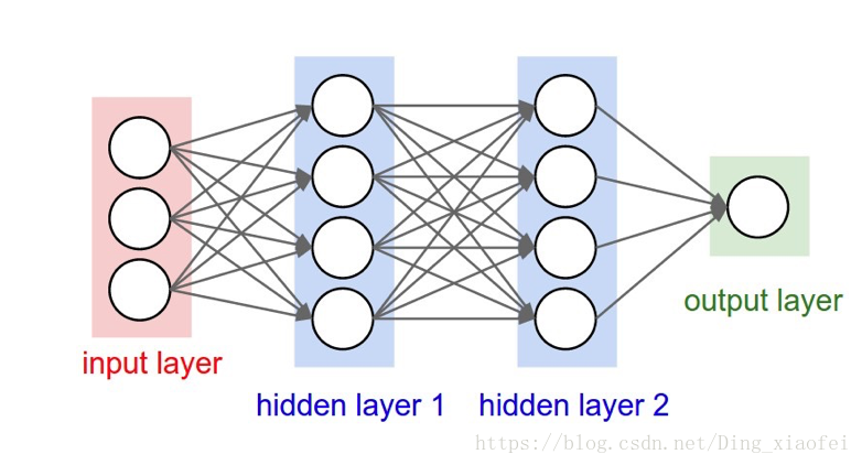
总算要进入我们的正题啦，这边先放一个神经网络的图，然后我们在引入我们需要解决的问题。

我们还是由我们的逻辑回归引入我们的神经网络，其实逻辑回归也是一种神经网络，但是它是没有深度的神经网络，作用的神经元也只有一个。解决的问题也很有局限，比如xor问题，逻辑回归是无法解决的。原因也很简单，你画出xor问题的点，它是无法通过一条线就把它分开的。

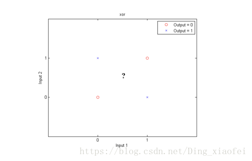
如图所示，大概我们只能给它画个圈来分类。因为它不再是线性可分的，这时候我就要想怎样才能组合特征给它搞出这个非线性的分割线呢。这时候我们的神经网络就闪亮登场啦。就想svm的核函数能够把数据点映射到高维空间，我们的深层神经网络也有着这样的魔力。

老规矩，代码先撸为敬。

# Lab 9 XOR
import tensorflow as tf
import numpy as np

tf.set_random_seed(777)  # for reproducibility
learning_rate = 0.1

x_data = [[0, 0],
          [0, 1],
          [1, 0],
          [1, 1]]
y_data = [[0],
          [1],
          [1],
          [0]]
x_data = np.array(x_data, dtype=np.float32)
y_data = np.array(y_data, dtype=np.float32)

X = tf.placeholder(tf.float32, [None, 2])
Y = tf.placeholder(tf.float32, [None, 1])

W1 = tf.Variable(tf.random_normal([2, 2]), name='weight1')
b1 = tf.Variable(tf.random_normal([2]), name='bias1')
layer1 = tf.sigmoid(tf.matmul(X, W1) + b1)

W2 = tf.Variable(tf.random_normal([2, 1]), name='weight2')
b2 = tf.Variable(tf.random_normal([1]), name='bias2')
hypothesis = tf.sigmoid(tf.matmul(layer1, W2) + b2)

# cost/loss function
cost = -tf.reduce_mean(Y * tf.log(hypothesis) + (1 - Y) *
                       tf.log(1 - hypothesis))

train = tf.train.GradientDescentOptimizer(learning_rate=learning_rate).minimize(cost)

# Accuracy computation
# True if hypothesis>0.5 else False
predicted = tf.cast(hypothesis > 0.5, dtype=tf.float32)
accuracy = tf.reduce_mean(tf.cast(tf.equal(predicted, Y), dtype=tf.float32))

# Launch graph
with tf.Session() as sess:
    # Initialize TensorFlow variables
    sess.run(tf.global_variables_initializer())

    for step in range(10001):
        sess.run(train, feed_dict={X: x_data, Y: y_data})
        if step % 100 == 0:
            print(step, sess.run(cost, feed_dict={
                  X: x_data, Y: y_data}), sess.run([W1, W2]))

    # Accuracy report
    h, c, a = sess.run([hypothesis, predicted, accuracy],
                       feed_dict={X: x_data, Y: y_data})
    print("\nHypothesis: ", h, "\nCorrect: ", c, "\nAccuracy: ", a)


'''
Hypothesis:  [[ 0.01338218]
 [ 0.98166394]
 [ 0.98809403]
 [ 0.01135799]]
Correct:  [[ 0.]
 [ 1.]
 [ 1.]
 [ 0.]]
Accuracy:  1.0
'''