Machine Learning - linear regression algorithm principle and the advantages and disadvantages

First, the principle of linear regression algorithm

　　Return for new data to predict, for example, to predict stock movements based on existing data. Here we talk about simple linear regression. Standards-based linear regression, may extend more linear regression algorithm.　

　　Suppose we find a best-fit linear equation: ,

　　　　For each sample point is , according to our linear equation, predictive value: which corresponds to the true value .

　　We hope and gap as small as possible, here we use the expression and the distance,

　　　　Consider all samples was:

　　Our goal is to make as small as possible, and so we have to find A, b , making as small as possible.

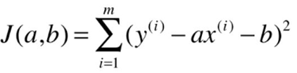
　　　　It is called loss function or utility function.

　　By analyzing the problems, loss of function or utility function to determine the problem, by optimizing the loss of function or utility function, to obtain the model of machine learning, which is half the routine parameter learning algorithm.

　　Seeking loss function may be converted into typical least-squares problem: minimize square error.

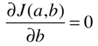
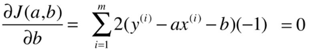
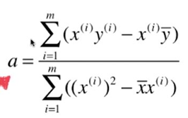
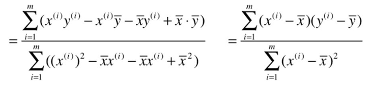
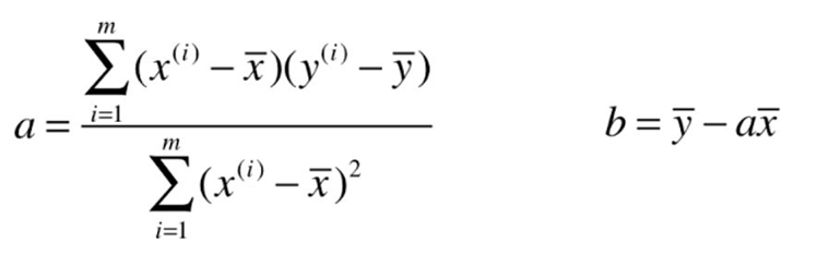
　　　　The process of solving the least squares method:

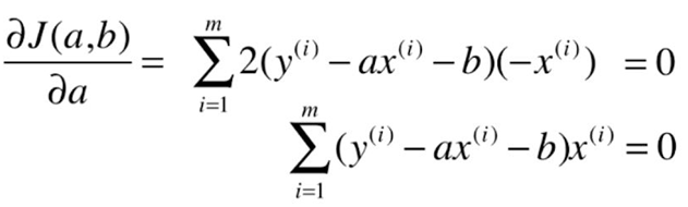
Goal: to find A, b , making as small as possible.

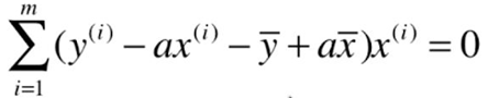
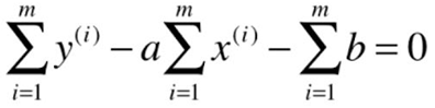
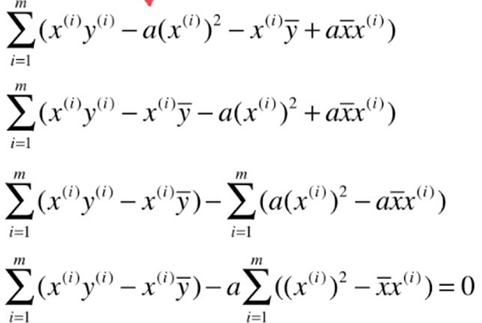
　　The general process:

假设输入数据集D有n个样本，d个特征，则：

D=\lgroup{ (x^{(1)},y_1) , (x^{(2)},y_2) ...(x^{(n)},y_n) } \rgroup

其中第

i

个样本表示为：

(x^{(i)},y_i)=(x_1^{(i)},x_2^{(i)},...x_d^{(i)},y_i)

线性模型通过建立线性组合进行预测。我们的假设函数为：

h_\theta(x_1,x_2,...x_d)=\theta_0+\theta_1x_1+\theta_2x_2+...+\theta_dx_d \qquad(1)

其中

\theta_0,\theta_1...\theta_d

为模型参数。
令

x_0=1

，

x^{(i)}=(x_1^{(i)},x_2^{(i)},...x_d^{(i)})

为行向量，令

X=\begin{bmatrix} x^{(0)}\\ x^{(1)}\\ \vdots\\ x^{(n)} \end{bmatrix}_{n \times d}， \theta=\begin{bmatrix} \theta_0\\ \theta_1\\ \vdots\\ \theta_d \end{bmatrix}_{d \times 1} ， Y=\begin{bmatrix} y_1\\ y_2\\ \vdots\\ y_n \end{bmatrix}_{n \times 1}

X

为

n \times d

维矩阵,

\theta

为

d \times 1

维向量，则假设函数(1)式可表示为：

h_\theta(X)=X\theta

损失函数为均方误差，即

J(\theta)=\frac{1}{2} (X\theta - Y)^T (X\theta - Y)

最小二乘法求解参数，损失函数

J(\theta)

对

\theta

求导：

\nabla J(\theta)=2X^T(X\theta-Y)

令

\nabla J(\theta)=0

，得

\theta=(X^TX)^{-1}X^TY

二、算法优缺点

　　优点：

　　　　（1）思想简单，实现容易。建模迅速，对于小数据量、简单的关系很有效；

　　　　（2）是许多强大的非线性模型的基础。

　　　　（3）线性回归模型十分容易理解，结果具有很好的可解释性，有利于决策分析。

　　　　（4）蕴含机器学习中的很多重要思想。

　　　　（5）能解决回归问题。

　　缺点：

　　　　（1）对于非线性数据或者数据特征间具有相关性多项式回归难以建模.

　　　　（2）难以很好地表达高度复杂的数据。

三、代码实现

　　1.简单的线性回归算法

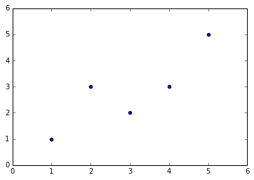
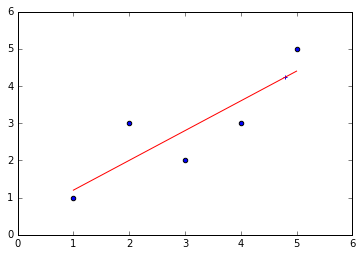
import numpy as np
import matplotlib.pyplot as plt

x=np.array([1,2,3,4,5],dtype=np.float)
y=np.array([1,3.0,2,3,5])
plt.scatter(x,y)

x_mean=np.mean(x)
y_mean=np.mean(y)
num=0.0
d=0.0
for x_i,y_i in zip(x,y):
    num+=(x_i-x_mean)*(y_i-y_mean)
    d+=(x_i-x_mean)**2
    a=num/d
    b=y_mean-a*x_mean
y_hat=a*x+b

plt.figure(2)
plt.scatter(x,y)
plt.plot(x,y_hat,c='r')
x_predict=4.8
y_predict=a*x_predict+b
print(y_predict)
plt.scatter(x_predict,y_predict,c='b',marker='+')

输出结果：

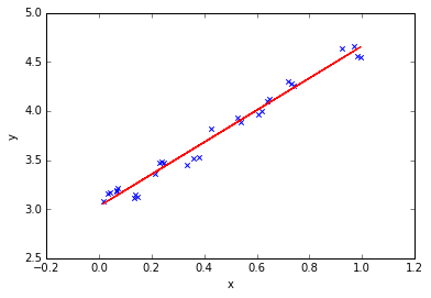
　　2.基于sklearn的简单线性回归

import numpy as np 
import matplotlib.pyplot as plt  
from sklearn.linear_model import LinearRegression  # 线性回归


# 样本数据集，第一列为x，第二列为y，在x和y之间建立回归模型
data=[
    [0.067732,3.176513],[0.427810,3.816464],[0.995731,4.550095],[0.738336,4.256571],[0.981083,4.560815],
    [0.526171,3.929515],[0.378887,3.526170],[0.033859,3.156393],[0.132791,3.110301],[0.138306,3.149813],
    [0.247809,3.476346],[0.648270,4.119688],[0.731209,4.282233],[0.236833,3.486582],[0.969788,4.655492],
    [0.607492,3.965162],[0.358622,3.514900],[0.147846,3.125947],[0.637820,4.094115],[0.230372,3.476039],
    [0.070237,3.210610],[0.067154,3.190612],[0.925577,4.631504],[0.717733,4.295890],[0.015371,3.085028],
    [0.335070,3.448080],[0.040486,3.167440],[0.212575,3.364266],[0.617218,3.993482],[0.541196,3.891471]
]


#生成X和y矩阵
dataMat = np.array(data)
X = dataMat[:,0:1]   # 变量x
y = dataMat[:,1]   #变量y


# ========线性回归========
model = LinearRegression(copy_X=True, fit_intercept=True, n_jobs=1, normalize=False)
model.fit(X, y)   # 线性回归建模
print('系数矩阵:\n',model.coef_)
print('线性回归模型:\n',model)
# 使用模型预测
predicted = model.predict(X)

plt.scatter(X, y, marker='x')
plt.plot(X, predicted,c='r')

plt.xlabel("x")
plt.ylabel("y")

输出结果：

系数矩阵:
[ 1.6314263]
线性回归模型:
LinearRegression(copy_X=True, fit_intercept=True, n_jobs=1, normalize=False)

Machine Learning - linear regression algorithm principle and the advantages and disadvantages

Guess you like