Popular understanding of linear regression
regression analysis
What is regression analysis? This is a concept from statistics. Regression analysis refers to a predictive modeling technique, which mainly studies the relationship between independent variables and dependent variables. Usually use lines/curves to fit the data points, and then study how to minimize the difference in distance from the curve to the data point.
For example, there are the following data

and then we fit a curve f(x):

The goal of regression analysis is to fit a curve so that the sum of the red lines in the figure is the smallest.
Linear regression (introduction)
Linear regression is a type of regression analysis.
- Assume that the target value (dependent variable) and the characteristic value (independent variable) are linearly related (that is, satisfy a multivariate linear equation, such as: f(x)=w1x1+…+wnxn+b.).
- Then construct the loss function.
- Finally, the parameters are determined by minimizing the loss function. (The most critical step)
Linear regression (detailed explanation)
According to the idea of introduction, the introduction is made with a simple one- variable linear regression (one-variable represents only one unknown independent variable).
There are n sets of data, independent variables x(x1,x2,...,xn), dependent variables y(y1,y2,...,yn), and then we assume the relationship between them is: f(x)=ax+b. Then the goal of linear regression is how to minimize the difference between f(x) and y, in other words, when the value of a and b is the closest to f(x) and y.
Here we have to solve another problem first, which is how to measure the difference between f(x) and y. In regression problems, the mean square error is the most commonly used performance metric in regression tasks (please check the mean square error by Baidu). Let J(a,b) be the difference between f(x) and y, that is,
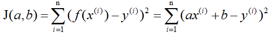
i represents the i-th group in the n groups of data.
Here J(a,b) is called the loss function. It can be clearly seen that it is a quadratic function, that is, a convex function ( the convex function here corresponds to the concave function of the Chinese textbook ), so it has a minimum value. When J(a,b) takes the minimum value, the difference between f(x) and y is the smallest, and then we can determine the values of a and b by taking the minimum value of J(a,b).
At this point, we can say that linear regression is all there is, but we still need to solve the most critical problem: determine the values of a and b .
Here are three methods to determine the value of a and b:
- Least squares method
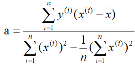
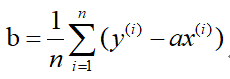
Since the loss function J(a,b) is convex, then take the partial derivative of J(a,b) with respect to a and b respectively, and make them zero to solve a and b. Here is the result directly: the


solution is:
-
Gradient descent method
First of all, you have to understand the concept of gradient: the original meaning of gradient is a vector (vector), which means that the directional derivative of a certain function ( the function is generally binary and above ) at that point is obtained along the direction The maximum value, that is, the function changes fastest along this direction (the direction of this gradient) at this point, and the rate of change is the largest (modulo this gradient).
When the function is a one-variable function, the gradient is the derivative. Here we use a simplest example to explain the gradient descent method, and then generalize the understanding of more complex functions.
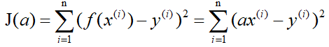
Still use the above example, there are n sets of data, independent variables x(x1,x2,...,xn), dependent variables y(y1,y2,...,yn), but this time we assume that the relationship between them is: f (x)=ax. Let J(a) be the difference between f(x) and y, that is,
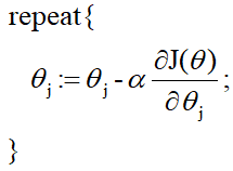
in the gradient descent method, we need to first assign a preset value to the parameter a, and then modify a little by little until J(a When taking the minimum value, determine the value of a. The formula of the gradient descent method is directly given below (where α is a positive number):

The meaning of the formula is explained below. The relationship between J(a) and a is shown in the figure below.
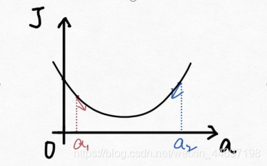
If the preset value for a is a1, then a is If the derivative of J(a) is negative, it is
also negative, so it

means that a moves a bit to the right. Then repeat this action until J(a) reaches the minimum value.
In the same way, if the preset value for a is a2, then the derivative of a with respect to J(a) is positive, which
means that a is shifted to the left. Then repeat this action until J(a) reaches the minimum value.
So we can see that no matter how much the preset value of a is taken, J(a) will always reach the minimum after multiple iterations of the gradient descent method.
Here is another chestnut in life. In the gradient descent method, assigning a preset value to a randomly is like you appear on a hillside randomly, and then you want to go to the lowest point of the valley in the fastest way, then you You have to judge where you should go for the next step. After taking a step, judge the direction of the next step again, and so on, you can go to the lowest point of the valley. And the α in the formula is called the learning rate, which can be understood in Chestnut as how big your step is. The larger the α, the larger the step. (In practice, the value of α cannot be too large or too small. Too large will cause the loss function J to approach the minimum value, and the next step will pass. For example, when you approach the lowest point of the valley, your step will be too large to step over. When we go back in the next step, we will step over again, and we will never reach the lowest point; if α is too small, the movement speed will be too slow, because of course we hope to ensure that we reach the lowest point as soon as possible. .)
At this point, you basically understand the idea of the gradient descent method, but in the chestnut we use the simplest case to explain, and in fact the gradient descent method can be extended to multiple linear functions, here is a direct formula , Understanding ( you need to have an understanding of the relevant knowledge of multivariate functions ) and the above chestnut have the same goal.
Assuming there are n sets of data, the relationship between the target value (dependent variable) and the characteristic value (independent variable) is:
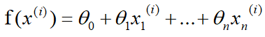
where i represents the i-th set of data, and the loss function is:
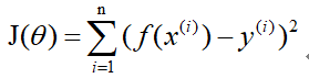
gradient descent method:
-
Normal equations
(knowledge of matrices are required here)
Normal equations are generally used in multiple linear regression, and you can understand why after reading it. So here is no longer a one-element linear regression.
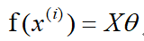
Similarly, assuming there are n sets of data, the relationship between the target value (dependent variable) and the characteristic value (independent variable) is:
where i represents the ith set of data, and the formula of the normal equation is directly given here: the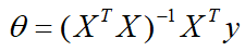
derivation process is as follows :
Remember the matrix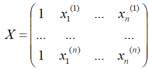
vector and
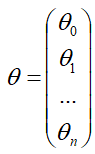

the
loss function is: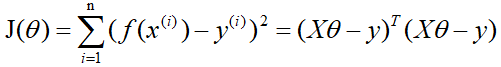
take the derivative of the loss function and set it to 0, if there is a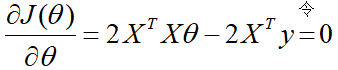
solution to get
this, all the coefficients θ are obtained. However, it should be noted that the normal equation
may appear as a singular matrix in practice, often because the eigenvalues are not independent . At this time, you need to filter the feature values to eliminate those feature values that have a linear relationship (for example, in the predicted housing price, feature value 1 represents the calculation of the house in feet, and feature value 2 represents the calculation of the house in square meters. At this time, the feature Value 1 and eigenvalue 2 only need to keep 1).
Well, the above is the explanation of linear regression (if it is really helpful for your understanding of linear regression, please give me a thumbs up, and also welcome to point out problems). Let me add my personal evaluation of the above three methods of determining the coefficient θ.
- Gradient descent method is universal, including more complex logistic regression algorithms can also be used, but for smaller amounts of data, its speed has no advantage
- The speed of the normal equation is often faster, but when the order of magnitude reaches a certain level, the gradient descent method is faster, because the normal equation needs to invert the matrix, and the time complexity for the inversion is the 3rd power of n
- The least squares method is generally seldom used. Although its idea is relatively simple, it is necessary to derivate the loss function and make it zero in the calculation process to solve the coefficient θ. But it is difficult for computers to implement, so the least square method is generally not used.