Sorting out differential equations (2)

Arrange differential equations

Example 1: \(y'=x^2+y^2\)    domain R: |x|≤1,|y|≤1, initial value (0,0), find the error between an approximate solution and the true solution No more than 0.05.

This is an unsolvable first-order differential equation, and we can only find its approximate solution

令\(f(x,y)=x^2+y^2\)

a=1,b=1，\(M=\max_R{f(x,y)}=\max_R(x^2+y^2)=2\)，\(h=\min\{a,{b\over M}\}={1\over 2}\)，\(L=\max{f_y'}=\max{2y}=2\)

Therefore \(|x|≤{1\over 2}\) , then the error between the nth approximate solution and the true solution is

\(|φ_n(x)-φ(x)|≤M⋅{L^nh^{n+1}\over (n+1)!}={2⋅2^n⋅({1\over 2})^{n+1}\over (n+1)!}={1\over (n+1)!}<0.05\)

Get n=3

It can be obtained from the initial value (0,0)

\(φ_0=0\)

\(φ_1=y_0+\int_{x_0}^xf(ξ,φ_0(ξ))dξ=\int_0^xξ^2dξ={x^3\over 3}\)

\(φ_2=y_0+\int_{x_0}^xf(ξ,φ_1(ξ))dξ=\int_0^x(ξ^2+{ξ^6\over 9})dξ={x^3\over 3} +{x^7\over 63}\)

\(φ_3=y_0+\int_{x_0}^xf(ξ,φ_2(ξ))dξ=\int_0^x(ξ^2+({ξ^3\over 3}+{ξ^7\over 63}) ^2)dξ=\int_0^x(ξ^2+{ξ^6\over 9}+{2ξ^{10}\over 189}+{ξ^{14}\over 3969})dξ\)

\(={x^3\over 3}+{x^7\over 63}+{2x^{11}\over 2079}+{x^{15}\over 59535}\)

This approximate solution is the approximate solution that meets the requirements.

Example 2: Picard sequence of y'=x+y+1, y(0)=0, and solve it by taking the limit

令f(x,y)=x+y+1

\(φ_0=0\)

\(φ_1=y_0+\int_{x_0}^xf(ξ,φ_0(ξ))dξ=\int_0^x(ξ+1)dξ={x^2\over 2}+x\)

\(φ_2=y_0+\int_{x_0}^xf(ξ,φ_1(ξ))dξ=\int_0^x(ξ+1+{ξ^2\over 2}+ξ)dξ={x^3\over 3!}+x^2+x\)

\(φ_3=y_0+\int_{x_0}^xf(ξ,φ_2(ξ))dξ=\int_0^x(ξ+1+{ξ^3\over 6}+ξ^2+ξ)dξ={x ^4\over 4!}+{x^3\over 3}+x^2+x\)

It can be obtained from the rules

\(φ_n={x^{n+1}\over (n+1)!}+2({x^n\over n!}+{x^{n-1}\over (n-1)!}+...+{x\over 2})={x^{n+1}\over (n+1)!}+2({x^n\over n!}+{x^{n-1}\over (n-1)!}+...+x+1)-x-2\)

\(\lim_{n->∞}φ_n(x)=φ(x)=2e^xx-2\)

is the true solution of the equation.

What needs to be explained here is

\(\lim_{n->∞}{x^{n+1}\over (n+1)!}=0\) , you can refer to Proposition 5 in the arrangement of differential equations for explanation

\(\lim_{n->∞}({x^n\over n!}+{x^{n-1}\over (n-1)!}+...+x+1)=e^ x\) , you can refer to two important limits in advanced mathematics

But in fact, this is a first-order linear non-homogeneous equation, which is solvable

P(x)=1,Q(x)=x+1

According to the general solution formula of the first-order linear non-homogeneous equation, we have

\(y=e^{∫P(x)dx}∫Q(x)e^{−∫P(x)dx}dx+Ce^{∫P(x)dx}=e^{\int1dx}\int(x+1)e^{-\int1dx}dx+Ce^{\int1dx}\)

\(=e^x\int{x+1\over e^x}dx+Ce^x=-e^x\int{x+1\over e^x}d(-x)+Ce^x=-e^x\int(x+1)d(e^{-x})+Ce^x\)

\(=-e^x[(x+1)e^{-x}-\int{e^{-x}d(x+1)}]+Ce^x=-e^x[(x+1)e^{-x}+\int{e^{-x}d(-x)}]+Ce^x\)

\(=-e^x[(x+1)e^{-x}+e^{-x}]+Ce^x\)

\(=-e^x(e^{-x}+xe^{-x}+e^{-x})+Ce^x=Ce^xx-2\)

Substituting y(0)=0, we get C=2, so the special solution that satisfies the initial conditions is

\(y=2e^x-x-2\)

• continuation of solution

1. \({dy\over dx}=x^2+y^2\)
2. y(0)=0

R：|x|≤1,|y|≤1

Here we know

\(|x|≤h={1\over 2}\)

If we increase the scope of the domain R, such as

R: |x|≤2,|y|≤2, at this time

 a=2,b=2，\(M=\max_R{f(x,y)}=\max_R(x^2+y^2)=8\)，\(h=\min\{a,{b\over M}\}={1\over 4}\)

Therefore

\(|x|≤h={1\over 4}\)

It can be seen that as the definition domain becomes larger, the solution interval will become smaller .

To overcome this shortcoming, we need to extend the solution .

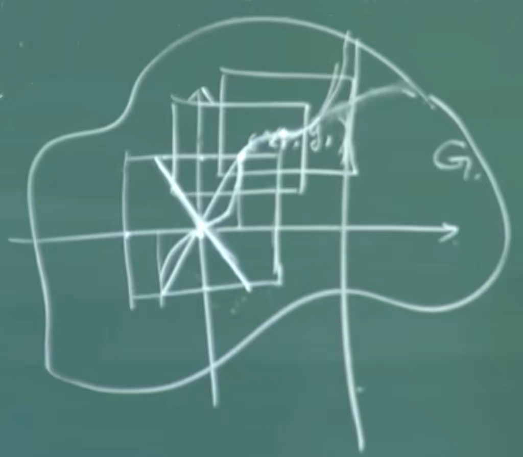
In the above figure, the solution of passing (0,0) is between \(-{1\over 2}\) and \({1\over 2}\) . When the function curve reaches \(({1\over 2 },1)\) , we take \(({1\over 2},1)\) as a new initial point, continue to use the existence and uniqueness theorem of the solution, and determine a new domain \ (R_1\) , the left side of \(({1\over 2},1)\) coincides with the original function curve, and a new section will extend on the right side of \(({1\over 2},1)\) Function curve of _ _ _ _ _ (x_0+h_1+h_2\) , when x reaches \(x_0+h_1+h_2\) , continue to make a bounded closed domain. If the function f(x,y) satisfies the Lipschitz condition with respect to y, then The existence and uniqueness theorem of linear solutions can be applied.

We have been doing this kind of extension, which can be extended to the left or right. Assuming that the bounded closed domain of \({dy\over dx}=x^2+y^2\) itself is G, It is possible to continue extending to the boundary of G, but sometimes it cannot reach the boundary. There may be a vertical line as shown in the picture above. When x reaches the vertical line, \({dy\over dx}=∞\ ) , then the function curve will be infinitely close to the upward extension of the vertical line.

This theorem is the continuation theorem of the solution . The maximum interval in which a solution can exist is called a saturated solution , that is, y=φ(x) cannot be extended to the left or right.

Here f(x,y) is a continuous function, that is, it satisfies the existence of solution, and it only needs to satisfy the local Lipschitz condition for y, which is weaker than the global Lipschitz condition. If y satisfies the global Lipschitz condition, it satisfies the Lipschitz condition at every point, so there is a continuation theorem of understanding.

Theorem 3: (The continuation theorem of the solution) If the right-hand function f(x,y) is continuous in the bounded closed domain G, and satisfies the local Lipschitz condition with respect to y, then

1. \({dy\over dx}=f(x,y)\)
2. \(y(x_0)=y_0\)

The solution can definitely be extended. In the direction of increasing x, y=φ(x) can be extended to \([x_0,d)\) . When x->d, the solution (x,φ(x)) tends to The boundary of G.

Corollary: If G is an unbounded area, in the continuation theorem, the solution y=φ(x) of \((x_0,y_0)\) has two continuation situations in the direction of increasing x. kind

1. \((x_0,∞)\)
2. \((x_0,d)\)   d is a finite number

φ(x) is unbounded.

Example 1: \({dy\over dx}={y^2-1\over 2}\) passes through the point (0,0), the existence interval of the solution of (ln2,-3).

Although this differential equation is a solvable equation with variable separation, we can see that we do not need to solve the equation here.

1. y=1
2. y=-1

are the two straight-line solutions of the equation

Let \(f(x,y)={y^2-1\over 2}\) , be a continuous function, and y satisfies the Lipschitz condition L=y, then the initial value (0,0) The solution must exist and be unique.

When |y|<1, f(x,y)<0, that is, \(y'={dy\over dx}<0\) , indicating that the solution y=φ(x) is monotonically decreasing. Observe its concavity and convexity through y''.

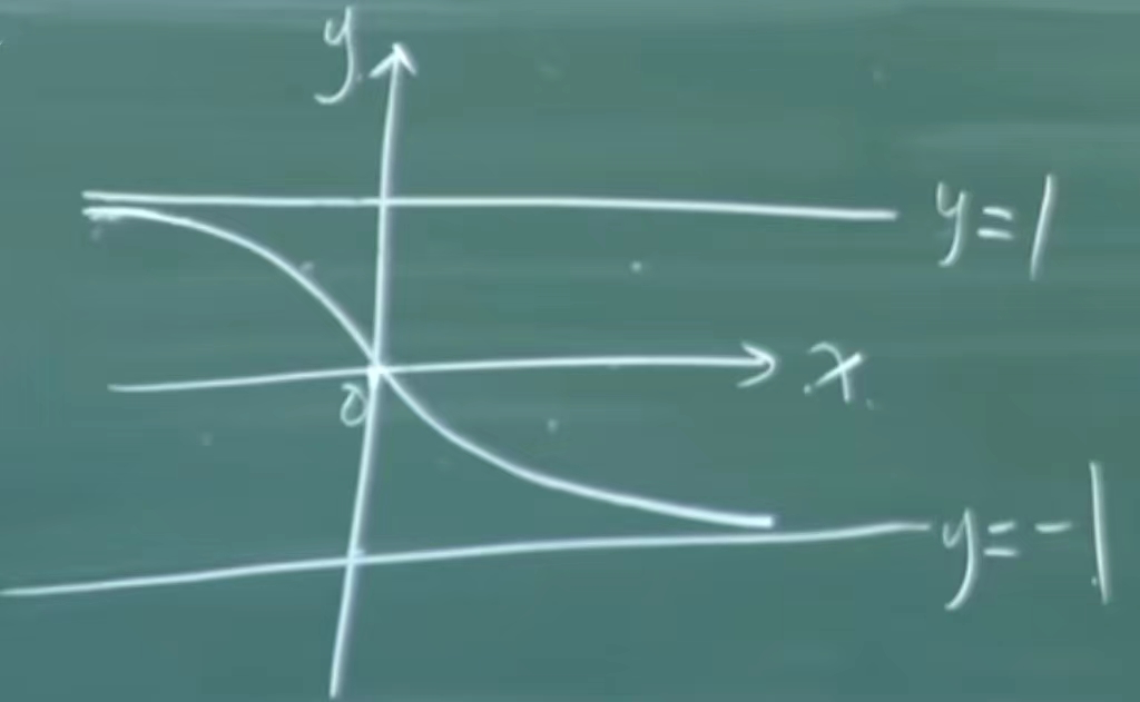
This is a monotonically decreasing curve that is infinitely close to y=1 when x<0, and infinitely close to y=-1 when x>0. The existence interval of the solution is (-∞, +∞), then according to

1. \({dy\over dx}={y^2-1\over 2}\)
2. y(0)=0

There is \(x\in(-​∞,+∞)\) , which is a saturated solution

Now let's look at the case of (ln2,-3) again. The solution passing this initial point also exists and is unique.    

Since \(y_0=-3\) , that is, \(|y|>1\) , f(x,y)>0, that is, \(y'={dy\over dx}>0\) , it means that the solution y =φ(x) is monotonically increasing.

Since the solution exists and is unique, the direction increasing from (ln2,-3) to x is close to y=-1 and cannot exceed y=-1, otherwise the solution will not be unique.

Starting from (ln2,-3) in the direction of x decreasing, as y decreases, \(y^2->∞\) , indicating that y'->∞ does not exist, and the function curve will infinitely approach downward to The y-axis, that is, the x value can only approach 0 but cannot reach 0, so

1. \({dy\over dx}={y^2-1\over 2}\)
2. y(ln2)=-3

There is \(x\in(0,+∞)\) , these two intervals are maximum intervals, not local intervals.

• Continuity and differentiability of solution with respect to initial values

Theorem 4: Suppose f(x,y) is continuous in the domain D and satisfies the Lipschitz condition with respect to y, y=φ(x) is

1. \({dy\over dx}=f(x,y)\)     a≤x≤b
2. \(y(x_0)=y_0\)

The solution of \(a≤x_0≤b\) , given any ε>0, there must be a positive number δ such that

\((x_1-x_0)^2+(y_1-y_0)^2≤δ^2\)

When, the equation satisfies

\(y(x_1)=y_1\)

It is also defined in the interval [a, b], and

\(|φ(x,x_1,y_1)-φ(x,x_0,y_0)|<ε\)

This is called continuous.

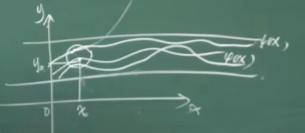
The above figure shows that within the neighborhood of a certain point (that is, the circle in the figure above), if any initial point is chosen, the resulting function will not differ too much from the original function.

Theorem 5: Differentiability of the solution with respect to the initial value

1. \({∂φ\over ∂x_0}=-f(x_0,y_0)e^{\int_{x_0}^x{∂f(x,φ)\over ∂y}dx}\)
2. \({∂φ\over ∂y_0}=e^{\int_{x_0}^x{∂f(x,φ)\over ∂y}dx}\)

When the solution is continuous with respect to the initial value and the above partial derivative formula is satisfied, the solution is still differentiable with respect to the initial value. The proof of this condition is more cumbersome, but it is the same as the principle of differentiability of functions. For the meaning of differentiability of functions, please refer to the definition of differential in Advanced Mathematics .

General theory of linear differential equations

Given n functions

\(x_1(t),x_2(t),x_3(t),...,x_n(t)\)

To determine whether these linear functions are linearly dependent or linearly independent (for information about linear correlation and linear independence, please refer to Linear correlation and linear independence in linear algebra ), we need to construct a new determinant

W(t)=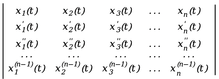

This is an n-order determinant, called the Wronsky determinant. For information about determinants, please refer to Determinants in Linear Algebra Sorting (3)

Theorem 2: If the function \(x_1(t),x_2(t),x_3(t),...,x_n(t)\) is linearly related on the definition interval [a,b], then W(t)= 0

Proof: If the functions \(x_1(t),x_2(t),x_3(t),...,x_n(t)\) are linearly related, then there is a set of constants that are not all 0 \(C_1,C_2,C_3, ...,C_n\) , such that

\(C_1x_1(t)+C_2x_2(t)+C_3x_3(t)+...+C_nx_n(t)=0\)

We can continuously find derivatives from 1 to n-1 at both ends according to the above formula, and we have

\(C_1x_1'(t)+C_2x_2'(t)+C_3x_3'(t)+...+C_nx_n'(t)=0\)

\(C_1x_1''(t)+C_2x_2''(t)+C_3x_3''(t)+...+C_nx_n''(t)=0\)

...

\(C_1x_1^{(n-1)}(t)+C_2x_2^{(n-1)}(t)+C_3x_3^{(n-1)}(t)+...+C_nx_n^{(n-1)}(t)=0\)

This is a system of homogeneous linear equations. Since \(C_1,C_2,C_3,...,C_n\) is not all 0, it means that the system of homogeneous linear equations about the unknown number \(C_i\) has non-zero solutions, homogeneous The necessary and sufficient condition for a system of linear equations to have a non-zero solution is that the value of the coefficient determinant is 0, that is, W(t)=0.

For Theorem 2, the converse is not true, such as two piecewise functions

1. \(x_1(t)=t^2\)      -1≤t<0
2. \(x_1(t)=0\)         0≤t≤1

as well as

1. \(x_2(t)=0\)     -1≤t<0
2. \(x_2(t)=t^2\)      0≤t≤1

On the interval [-1,0), W(t)= =0;

On the interval [0,1], W(t)= =0

Although W(t) is equal to 0 on [-1,1], now looking at the function itself, there are two constants \(C_1,C_2\) , such that

On the interval [-1,0), \(C_1t^2+C_20=0\)

\(C_1t^2=0\) , since \(t≠0\) , only \(C_1=0\)

On the interval [0,1], \(C_10+C_2t^2=0\)

\(C_2t^2=0\) , although t can be equal to 0 here, when 0<t≤1, the equation to be established is also valid, and we have to \(C_2=0\)

Here we have \(C_1=C_2=0\) , all of them are 0, then \(x_1(t) and x_2(t)\) are linearly independent, so Theorem 2 does not hold in reverse. But if \(W(t)≠0\) , it must be linearly independent.

Theorem 3: \(x_1(t),x_2(t),x_3(t),...,x_n(t)\) is a linear higher-order differential equation

\({d^nx\over dt}+a_1(t){d^{n-1}x\over dt^{n-1}}+...+a_{n-1}(t){dx\over dt}+a_n(t)x=0\)

solution, then \(x_i(t)\) is linearly independent, then W(t) is not equal to 0 at any point on this interval [a, b], \(W(t)≠0\) , for ∀ t ∈[a,b].

Proof: Suppose \(∃ t_0∈[a,b]\)      st \(W(t_0)=0\)

\(W(t_0)=\)=0

At this point we can construct a system of equations

1. \(C_1x_1(t_0)+C_2x_2(t_0)+C_3x_3(t_0)+...+C_nx_n(t_0)=0\)
2. \(C_1x_1'(t_0)+C_2x_2'(t_0)+C_3x_3'(t_0)+...+C_nx_n'(t_0)=0\)
3. \(C_1x_1''(t_0)+C_2x_2''(t_0)+C_3x_3''(t_0)+...+C_nx_n''(t_0)=0\)
4. ...
5. \(C_1x_1^{(n-1)}(t_0)+C_2x_2^{(n-1)}(t_0)+C_3x_3^{(n-1)}(t_0)+...+C_nx_n^{(n-1)}(t_0)=0\)

This is a set of homogeneous linear equations with \(C_1,C_2,C_3,...,C_n\) as unknowns, and the value of the coefficient determinant of this homogeneous linear equation is equal to 0, indicating that the homogeneous Systems of linear equations have non-zero solutions. We assume that this set of non-zero solutions is \(C_1^*,C_2^*,C_3^*,...,C_n^*\) , thus constructing a new solution to the original equation

\(x(t)=C_1^*x_1(t)+C_2^*x_2(t)+C_3^*x_3(t)+...+C_n^*x_n(t)\)

This is a linear combination. For linear combinations, please refer to Linear Combinations in Linear Algebra.

Since \(x_1(t),x_2(t),x_3(t),...,x_n(t)\) is the solution of the original equation, according to the principle of superposition of solutions , x(t) is also the solution of the original equation .

When \(t=t_0\) , then there is

\(x(t_0)=C_1^*x_1(t_0)+C_2^*x_2(t_0)+C_3^*x_3(t_0)+...+C_n^*x_n(t_0)=0\)

The derivatives of each order also satisfy the system of equations we constructed. It can be seen from the original equation that x(t)=0 is also the solution of the original equation. They all satisfy the initial conditions of the solution (  with \(C_1,C_2,C_3,.. .,C_n\) is a system of homogeneous linear equations with unknown numbers), due to the uniqueness of the solution

1. \(x(t)=C_1^*x_1(t)+C_2^*x_2(t)+C_3^*x_3(t)+...+C_n^*x_n(t)\)
2. x(t)=0

contradictory, so there is

\(C_1^*x_1(t)+C_2^*x_2(t)+C_3^*x_3(t)+...+C_n^*x_n(t)=0\)

And \(C_1^*,C_2^*,C_3^*,...,C_n^*\) is a non-zero solution, indicating that \(x_1(t),x_2(t),x_3(t),..., x_n(t)\) is linearly related, which contradicts the linear independence between \(x_i(t)\) . It is proved. 

General solution structure of linear homogeneous equations

According to Theorem 3, we know that the higher-order linear differential equation

\({d^nx\over dt}+a_1(t){d^{n-1}x\over dt^{n-1}}+...+a_{n-1}(t){dx\over dt}+a_n(t)x=0\)

The n solutions are \(x_1(t),x_2(t),x_3(t),...,x_n(t)\)

When \(t=t_0\) , we construct

1. \(x_1(t) \)        \(x_1(t_0)=1\)     \(x_1'(t_0)=0\)       \(x_1''(t_0)=0\)       ...        \(x_1^{(n-1)}(t_0)=0\)
2. \(x_2(t) \)        \(x_2(t_0)=0\)     \(x_2'(t_0)=1\)       \(x_2''(t_0)=0\)       ...        \(x_2^{(n-1)}(t_0)=0\)
3. \(x_3(t) \)        \(x_3(t_0)=0\)     \(x_3'(t_0)=0\)       \(x_3''(t_0)=1\)       ...        \(x_3^{(n-1)}(t_0)=0\)
4. ...
5. \(x_n(t) \)        \(x_n(t_0)=0\)     \(x_n'(t_0)=0\)       \(x_n''(t_0)=0\)       ...        \(x_n^{(n-1)}(t_0)=1\)

These are x(t) that satisfy the following initial conditions. By their Wronski determinant

\(W(t_0)=\)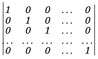\(=1≠0\)

It can be seen that as long as there is any point \(W(t_0)≠0\) , according to the inverse proposition of Theorem 3, this set of functions \(x_1(t),x_2(t),x_3(t),..., x_n(t)\) is linearly independent

Theorem 4: Higher-order linear differential equations

\({d^nx\over dt}+a_1(t){d^{n-1}x\over dt^{n-1}}+...+a_{n-1}(t){dx\over dt}+a_n(t)x=0\)

There must exist n linearly independent solutions.

Theorem 5: (General solution structure) if \(x_1(t),x_2(t),x_3(t),...,x_n(t)\) is

\({d^nx\over dt}+a_1(t){d^{n-1}x\over dt^{n-1}}+...+a_{n-1}(t){dx\over dt}+a_n(t)x=0\)

n linearly independent solutions, then the linear combination of these n linearly independent solutions

\(x(t)=C_1x_1(t)+C_2x_2(t)+C_3x_3(t)+...+C_nx_n(t)\)

is the general solution to the equation.

Proof: According to the principle of superposition of solutions, x(t) is the solution of the equation,

The Wronsky determinant composed of the coefficients of its unknowns \(C_1,C_2,C_3,...,C_n\) and \(x_1(t),x_2(t),x_3(t),..., x_n(t)\) is linearly independent, then we have

W(t)=\(≠0\)

again

\({∂(x,x',x'',...,x^{(n-1)})\over ∂(C_1,C_2,C_3,...,C_n)}=W(t) ≠0\) , according to the converse proposition of Theorem 2

It shows that \(C_1,C_2,C_3,...,C_n\) is linearly independent, and it is proved.

Here \({∂(x,x',x'',...,x^{(n-1)})\over ∂(C_1,C_2,C_3,...,C_n)}\) means The determinant composed of the partial derivatives of each order of the function x (including \(x_1,x_2,x_3,...,x_n\)) to C (including \(C_1,C_2,C_3,...,C_n\)) .

This shows that \({d^nx\over dt}+a_1(t){d^{n-1}x\over dt^{n-1}}+...+a_{n-1}(t) The solution space of {dx\over dt}+a_n(t)x=0\) constitutes an n-dimensional linear space, and its n linearly independent solutions can be used as a set of bases of the solution space. If this set of solutions satisfies

，

Then this set of solutions is called the basic solution set of the original equation .

But this is not the only way we can construct the solution to the original equation. As long as the value of this set of determinants is 1, linear independence can be satisfied , for example

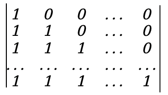\(=1≠0\)

This is a lower triangular determinant. The initial conditions have changed, so the solution x(t) has also changed, but at the same time x(t) is still linearly independent, that is, the basic solution group is not unique . but satisfied

The basic ungrouping of is called the standard basic ungrouping .

Example 1: The solutions of x''-x=0 are \(e^t\) and \(e^{-t}\) respectively , and the general solution is \(x(t)=C_1e^t+C_2e^{- t}\) , find the solution to the equation when x(0)=1,x'(0)=0 and x(0)=0,x'(0)=1.

From \(x(t)=C_1e^t+C_2e^{-t}\) , we get

\(x'(t)=C_1e^t-C_2e^{-t}\)

When t=0, x(0)=1,x'(0)=0

1. \(C_1+C_2=1\)
2. \(C_1-C_2=0\)

得\(C_1={1\over 2}\),\(C_2={1\over 2}\)

At this time, it is recorded as \(x_1(t)\) , then

\(x_1(t)={1\over 2}e^t+{1\over 2}e^{-t}={1\over 2}(e^t+e^{-t})\)

When t=0, x(0)=0,x'(0)=1

1. \(C_1+C_2=0\)
2. \(C_1-C_2=1\)

 得\(C_1={1\over 2}\),\(C_2=-{1\over 2}\)

At this time, it is recorded as \(x_2(t)\) , then

\(x_2(t)={1\over 2}e^t-{1\over 2}e^{-t}={1\over 2}(e^t-e^{-t})\)

Depend on

1. \(x_1(t)={1\over 2}(e^t+e^{-t})\)
2. \(x_2(t)={1\over 2}(e^t-e^{-t})\)

have to

W(t)=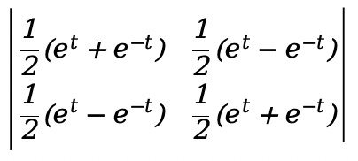\(=1≠0\)

It can be seen that \(x_1(t)\) and \(x_2(t)\) are linearly independent, so using these two solutions as the standard basic solution set, the general solution of the equation is

\(x(t)=C_1{1\over 2}(e^t+e^{-t})+C_2{1\over 2}(e^t-e^{-t})={1\over 2}[(C_1+C_2)e^t+(C_1-C_2)e^{-t}]\)

Let \(C_1^*={1\over 2}(C_1+C_2)\) , \(C_2^*={1\over 2}(C_1-C_2)\) , then

\(x(t)=C_1^*e^t+C_2^*e^{-t}\)

Although the above formula is very similar to \(x(t)=C_1e^t+C_2e^{-t}\) in form , they are not the same basic solution group. From here we can see that the standard basic solution set is not necessarily the most concise set of solutions.

Reducible second-order differential equations

There are only a few special types of reducible second-order differential equations

• \({d^2y\over dx^2}=f(x)\)型

Solving this type of second-order differential equation requires only two integrations

\({dy\over dx}=\int{f(x)dx}+C_1\)

\(y=\int{(\int{f(x)dx})dx}+C_1x+C_2\)

This is the general solution to this type of equation.

Example 1: \({d^2y\over dx^2}={1\over cos^2x}\) , when \(x_0={π\over 4}\) , \(y_0={ln2\over 2}\) , \(y_0'=1\)

\({dy\over dx}=tanx+C_1\)      (Here you can refer to the derivation of the tangent function in Advanced Mathematics )

Because  when \(x_0={π\over 4}\) , \(y_0'=1\) , so

\(1=tan{π\over 4}+C_1\)

\(1=1+C_1\)

\(C_1=0\)

Therefore

\({dy\over dx}=tanx\)

\(y=-ln|cosx|+C_2\)       (Here you can refer to the derivation of the integral formula of tangent in the arrangement of differential equations )

Because  when \(x_0={π\over 4}\) , \(y_0={ln2\over 2}\) , so

\({ln2\over 2}=-ln|cos{π\over 4}|+C_2\)

\({ln2\over 2}=-ln|{1\over \sqrt2}|+C_2\)

\({ln2\over 2}=ln\sqrt2+C_2\)

\(C_2=0\)

Therefore

\(y=-ln|cosx|\)

is the special solution of the original equation

• \({d^2y\over dx^2}=f(x,{dy\over dx})\)型

This type of equation does not obviously contain y, referred to as not containing y obviously, and is reduced in order through the variable substitution method.

Let \({dy\over dx}=p\) , then \({d^2y\over dx^2}={dp\over dx}\) , the original equation becomes

\({dp\over dx}=f(x,p)\)

Let the solution of this new equation be

\(p=φ(x,C_1)\)

but

\({dy\over dx}=φ(x,C_1)\)

The general solution of the original equation is

\(y=\int{φ(x,C_1)dx}+C_2\)

Example 2: \((1+x^2){d^2y\over dx^2}=2x{dy\over dx}\)

Let \({dy\over dx}=p\) , then \({d^2y\over dx^2}={dp\over dx}\) , the original equation becomes

\((1+x^2){dp\over dx}=2xp\)

Separate the variables and get

\({dp\over p}={2x\over 1+x^2}dx\)

Integral at both ends

\(\int{dp\over p}=\int{2x\over 1+x^2}dx\)

\(ln|p|=\int{{1\over 1+x^2}d(1+x^2)}\)

\(ln|p|=ln|1+x^2|+ln|C_1|\)

\(ln|p|=ln(|1+x^2|⋅|C_1|)\)

\(p=C_1(1+x^2)\)

Right now

\({dy\over dx}=C_1(1+x^2)\)

\(y=\int{C_1(1+x^2)dx}+C_2\)

\(y=C_1(x+{x^3\over 3})+C_2\)

is the general solution of the original equation

• \({d^2y\over dx^2}=f(y,{dy\over dx})\)型

This type of equation does not obviously contain x, referred to as not explicitly containing x, and is also reduced in order through variable substitution.

Let \({dy\over dx}=p\) , then \({d^2y\over dx^2}={dp\over dx}={dp\over dy}⋅{dy\over dx}=p {dp\over dy}\) , the original equation becomes

\(p{dp\over dy}=f(y,p)\)

Let the solution of this new equation be

\(p=φ(y,C_1)\)

but

\({dy\over dx}=φ(y,C_1)\)

separate variables

\({dy\over φ(y,C_1)}=dx\)

Integral at both ends

\(\int{dy\over φ(y,C_1)}=\int{dx}\)

Example 3: \(({dy\over dx})^2-y{d^2y\over dx^2}=0\)

Let \({dy\over dx}=p\) , then \({d^2y\over dx^2}={dp\over dx}={dp\over dy}⋅{dy\over dx}=p {dp\over dy}\) , the original equation becomes

\(p^2-yp{dp\over dy}=0\)

\((p-y{dp\over dy})p=0\)

So there is

1. \(p-y{dp\over dy}=0\)
2. p=0

From formula 1

\(p=y{dp\over dy}\)

separate variables

\({dy\over y}={dp\over p}\)

Integral at both ends

\(\int{dy\over y}=\int{dp\over p}\)

\(ln|p|=ln|y|+ln|C_1|\)

\(p=C_1y\) , p=0 is also a solution

That is the case of \(C_1=0\) , \(C_1\) can be any constant, in this case

\(p=C_1y\) is the general solution of \((py{dp\over dy})p=0\)

Right now

\({dy\over dx}=C_1y\)

separate variables

\({dy\over y}=C_1dx\)

Integral at both ends

\(\int{dy\over y}=\int{C_1dx}\)

\(ln|y|=C_1x+ln|C_2|\)

\(ln|y|=lne^{C_1x}+ln|C_2|\)

\(y=C_2e^{C_1x}\)

y=0 is also a solution, which is the case of the above formula \(C_2=0\)

Therefore

\(y=C_2e^{C_1x}\) is the general solution of the original equation, \(C_1,C_2\) is any constant

Google donated $1 million to the Rust Foundation to improve the interoperability between Rust and C++. The web engine project "Servo", which was abandoned by Mozilla, will be reborn in 2024. The father of the Go language summarizes the success factors: the mascot is indispensable jQuery 4.0 .0 beta released open source daily: "Small but beautiful" Tauri has supported Android and iOS; Apple's open source Pkl Google Bard was renamed Gemini, free independent APP Vite 5.1 was officially released, front-end construction tool gallery system PicHome 2.0.1 released Java tool set Hutool-5.8.26 is released, I wish you all the best. The large open source model MaLA-500 is released, supporting 534 languages.

{{o.name}}

{{m.name}}