Table of contents
1. Exponential growth model (Malthus population model)
[Advantages and disadvantages of the model]
2. Population model that blocks growth (Logistic model)
2. Special analysis on the Logistic model
2.1 The fastest growing point of population speed
Table 1 below gives the U.S. demographic table (unit: million) in the past two centuries. We established a mathematical model and tested it, and finally used it to predict the U.S. population in 2010.
| Year |
1790 |
1800 |
1810 |
1820 |
1830 |
1840 |
1850 |
1860 |
| population |
3.9 |
5.3 |
7.2 |
9.6 |
12.9 |
17.1 |
23.2 |
31.4 |
| Year |
1870 |
1880 |
1890 |
1900 |
1910 |
1920 |
1930 |
|
| population |
38.6 |
50.2 |
62.9 |
76.0 |
92.0 |
106.5 |
123.2 |
|
| Year |
1940 |
1950 |
1960 |
1970 |
1980 |
1990 |
2000 |
|
| population |
131.7 |
150.7 |
179.3 |
204.0 |
226.5 |
251.4 |
281.4 |
Table 1 U.S. population statistics, units: millions
1. Exponential growth model (Malthus population model)
Reverend Thomas Robert Malthus (February 13, 1766 - December 23, 1834). British clergyman, demographer, and economist. Famous for his population theory. In "On Population" (1798), it was pointed out that the population grows in a geometric progression while living resources can only grow in an arithmetical progression, so it will inevitably lead to famine, war and disease; it calls for decisive measures to be taken to curb the birth rate. His theory had an impact on Ricardo.
[Model Assumptions]
- The population growth rate is constant
- The absolute growth of population per unit time is proportional to the current population
- The total population changes continuously over time
【Symbol Description】

【Model creation】
The total population at time t is x(t). For a region or country, the number of x(t) is very large and can be regarded as a differentiable function.
Remember that at the initial time t=0, the total population is x0. According to assumption (2), from t to t+Δt, the increase in population is proportional to the product of x(t) and Δt, that is
Let Δt→0, get the differential equation of x(t)  [2.1]
[2.1]
Variable separation is easy to find  [2.2]
[2.2]
[2.2] is called the exponential growth model, also called the Malthus population model.
【Parameter Estimation】
In order to make better use of the data and linear fitting parameters in Table 1, take the logarithm of both sides of [2], and we have
Assume y=lnx, a=lnx0, then y=a+rt【3】
The purpose of this type of model is to forecast. The accuracy of the prediction cannot be completely determined by the model itself and needs to be tested with actual data. Therefore, when fitting data, the first 2/3 of the data are generally used to fit the parameters (self-appointed tutors supervise learning), and the last 1/3 of the data are used to test the usability of the model. If the data itself is small, it also means that there is too little information available, and the credibility of the model is inherently low.
Use the first 12 data and use matlab software to do straight line fitting.
clear
A=xlsread('d:\Arenkou.xlsx');
A=A';
t=A(:,1);x=A(:,2);
t1=t(1:12);y=log(x(1:12));
[b,bt,r,rt,st]=regress(y,[ones(length(y),1),t1]);
x0=exp(b(1));r=b(2);
The forecast formula is obtained:
![]() 【4】
【4】
Figure 2 is a comparison of theoretical values (line) and actual values (*) for the first 12 years. It can be seen that this model can basically describe the population growth of the United States before the 19th century. This is basically consistent with hypothesis (1), that is, the population growth rate is constant.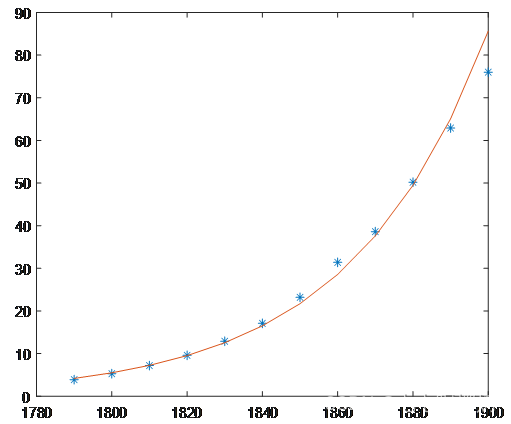
Figure 2 Exponential growth model fitting diagram (1790-1900)
Figure 3 is a comparison of theoretical values (line) and actual values (*) for all years. As can be seen from the figure, after entering the 20th century, the U.S. population growth has slowed down, and the model is no longer suitable. 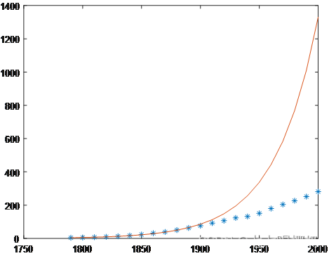
Figure 3 Exponential growth model fitting diagram (1790-2000)
[Analysis of error causes]
Use the form of difference quotient to define the growth rate, that is,  [5]
[5]
Substitute the data in Table 1 into [5] to obtain r(k), and plot it in Figure 4.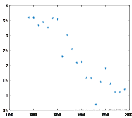
Figure 4 Time-growth rate scatter plot
It can be seen from Figure 4 that although the growth rate swings, there is a clear downward trend in the growth rate as the population grows. It can also be seen that the growth rate around 1930 was extremely small (due to the Great Depression of 2029).
[Advantages and disadvantages of the model]
1. Advantages
- The model is simple and easy to understand and calculate
- As can be seen from the first picture, the Malthus population model fits well in the short term, and the short-term prediction error is not very large.
2. Disadvantages
- As can be seen from the second picture, the Malthus model cannot make medium and long-term predictions, and the error is large.
- From
the looks of it, this is simply impossible, indicating that there are fatal flaws in the model assumptions.
3. Correction plan
Modify the growth rate from being a constant to the growth rate decreasing as the population increases.
2. Population model that blocks growth (Logistic model)
From the conclusion in Figure 4, we know that the growth rate will decrease with population growth. The real reason is that natural resources, environmental conditions and other conditions that human beings rely on for survival hinder population growth. As the population increases, the blocking effect becomes greater. .
[Model Assumptions]
- Population changes continuously over time
- There is an upper limit to the total population under a certain environment, that is, the maximum population xm
- The growth of population per unit time is equal to the current population × the current population growth rate
- The population growth rate at a certain time is a linear decreasing function of the population at that time
- When the population reaches maximum load, the growth rate is 0
【Symbol settings】
【Model creation】
1. Construct the model
The growth rate decreases as the population increases. Let's set it as r(x), which is the decreasing function of x. The simplest and most direct expression is a linear function.
![]() 【6】
【6】
where r is called the inherent growth rate, the maximum growth rate when x=0, and s is the retardation coefficient. It may be assumed that when x=xm, that is, when the population reaches the maximum load, the growth rate is 0, that is, [7  ]
]
Substituting [7] into [6], we get  [8]
[8]
According to the assumption [3], there is  [9]
[9]
In [9], dx/dt indicates that the actual growth rate of the population is divided into two parts. rx increases with the increase of population, and (1-x/xm) decreases with the increase of population. That is, population growth is the result of the joint action of two factors. . [9] The growth model reflected is called the retarded growth model, also known as the Logistic model.
Most of the biological population models with limited resources can use this model to describe the changing laws of the population; the production models and marketing models of many products also meet this law.
2. Special analysis on the Logistic model
2.1 The fastest growing point of population speed
Since the population growth rate (variable) decreases as the population size (variable) increases,  we can derive x from both sides by deriving
It can be seen that ![]() when x<xm/2, it increases monotonically; when x>xm/2, it decreases monotonically; when x=xm/2, the population change rate reaches the maximum. As shown in Figure 5.
when x<xm/2, it increases monotonically; when x>xm/2, it decreases monotonically; when x=xm/2, the population change rate reaches the maximum. As shown in Figure 5.
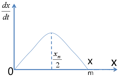
Figure 5 Logistic model dx/dt-x curve
2.2 Logistic model curve
It is  known that the population x(t) is a monotonically increasing function of time t, and since
F
Let's assume x(t0)=xm/2, then x(t) is a concave function when t<t0; x(t) is a convex function when t>t0. As shown in Figure 6.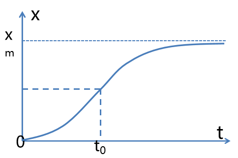
Figure 6 Logistic model xt curve (also known as s-shaped curve)
【Model Solving】
 【9】
【9】
[9] is a differential equation with variable separation. The specific solution obtained by solving it is
 【10】
【10】
The following conclusion can be obtained from the expression of [10]:
(1)![]()
(2)
Draw the curves obtained in the three cases of x0 in the same coordinate system, and the results are shown in Figure 7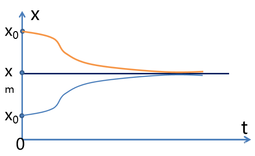
Figure 7 Schematic diagram of the population curve changing with different initial values x0
【Parameter Estimation】
 【10】
【10】
In the original data in Table 1, t is large, and it is the independent variable of the exponential function, which easily leads to extreme calculations. After the transformation, it becomes the following model.
 【11】
【11】
Using the first 21 data in Table 1, call least squares curve fitting in matlab, and get xm=397.2117;x0=7.1100;r=0.2255
The predicted population value of the United States in 2000 is  =268.08 (millions)
The relative prediction error reaches 4.63%.

Figure 8 xt fitting of the logistic model with the first 21 data Figure 9 xt fitting of the logistic model with the first 9 data removed
 = 277.9145 (according to the prediction in Figure 9)
The relative prediction error is 1.23%, which is better than the prediction in Figure 8. As can be seen from Figure 9, the error in the early stage is large. This also shows that the current data of biological populations are greatly affected by recent history and have little long-term impact.